Prerequisites: Trees, Graphs. It is recommended to review those chapters from BCtCI before reading this one.

Introduction

In this chapter, we will learn about a simple and elegant data structure known as the union–find or disjoint-set data structure. It is not part of most languages' built-in libraries because it is not as universally useful as data structures like arrays and maps, but in the right circumstances, it makes certain problems much easier.

We will learn to recognize when to use it, how to implement it from scratch quickly in an interview, and how to design efficient algorithms with it.

Like most data structures, the union–find data structure stores a set of elements (of any type, like numbers or strings), which can be added with a method add(x). The special feature of the union–find data structure is that each element belongs to a group or set. The two main operations have to do with these groups.

• The find(x) method returns the group containing x
• The union(x, y) method combines the groups containing x and y into a single group with all the elements of the two groups—similar to the union method of sets.

Besides add(), these are the main methods in the data structure—hence the unimaginative name "union–find."

Of the three methods, find() is the only one that returns something, so we should talk about its return type. That is, what does it mean to return "the group of an element"?

We could return the list of all the elements in the group. However, since all elements could belong to the same group, it would be expensive to return the list. Instead, what we want is to return something concise, like a unique identifier of the set. The key idea of the union–find data structure is to use one of the elements in the group as the group identifier. This way, find(a) only needs to return one element in the group containing a instead of all of them. We call this element the representative of the group. For instance, if one of the sets is {a, b, d}, then any of the three elements could be the representative. It doesn't matter which; the only thing that matters is that when you call find(a), find(b), or find(d), you will get that same representative.

This may seem peculiar at first, but we'll see how it is useful when we look at the applications.

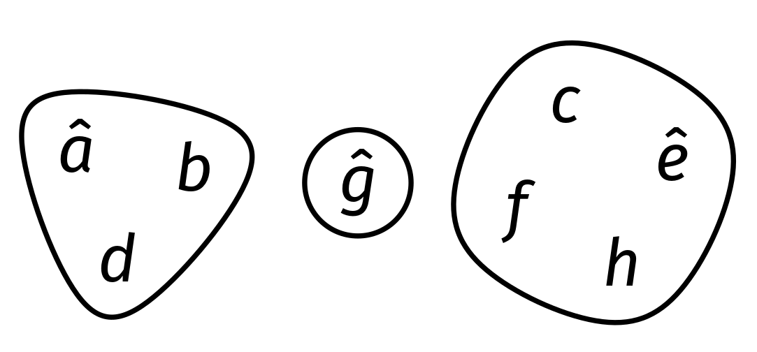
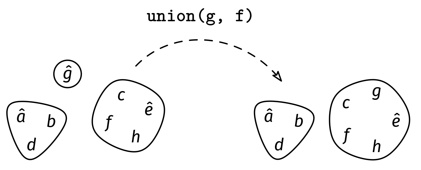
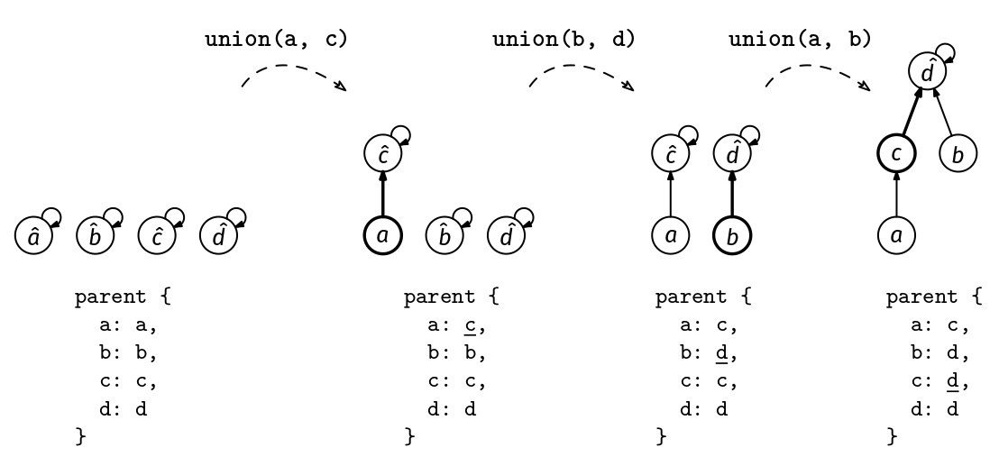
When an element x is added with add(x), we put it in a group all by itself, and thus x also becomes the representative of that set (like g in Figure 1). When sets are joined together with the union() method, the representative of either group is chosen as the representative of the new combined group.

UnionFind API:

add(x):      adds element x in a group by itself
find(x):     returns the representative of the set containing x
union(x, y): combines the set of x and y into a single set

In this chapter, we will show how to implement all these operations very efficiently—in essentially constant time. Before that, let's give an example of how a data structure with this API can be useful to solve a problem.

Recall Problem 9: First Time All Connected from the Graphs Chapter:

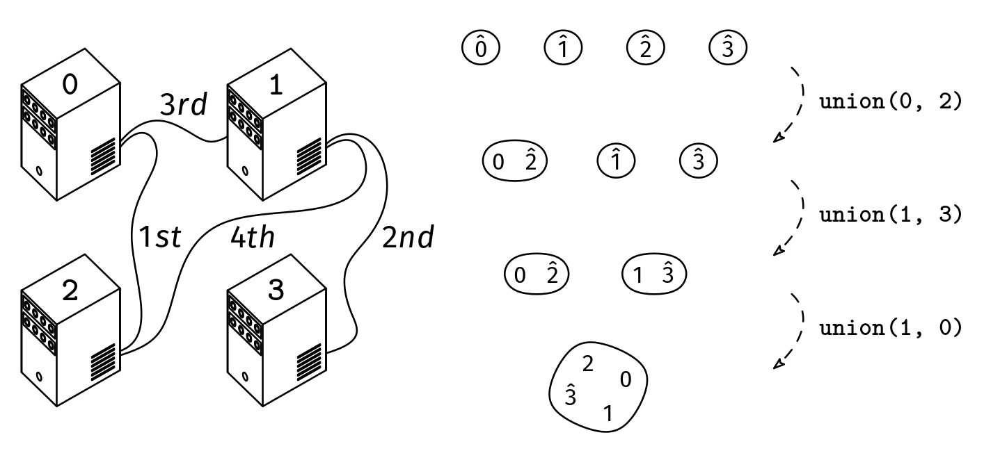
We are given n ≥ 2, the number of computers in a data center. The computers are identified with indices from 0 to n-1. We are also given a list, cables, of length m where each element is a pair [x, y], with 0 ≤ x,y < n, indicating that we should connect the computers with indices x and y with a cable. If we add the cables in the order of the list, at what point will all the computers be connected (meaning that there is a path of cables between every pair of computers)? Return the index of the cable in cables after which all the computers are connected or -1 if that never happens.

Example: n = 4, cables = [[0, 2], [1, 3], [1, 0], [1, 2]]
Output: 2. The computers become all connected with the cables at indices 0, 1, and 2.

Assume that V < 10^4 and E < 10^5.

We saw how to solve this problem in O((n + m) * log m) time using the guess-and-check binary search technique (see the Binary Search chapter) and a graph DFS.

We can get a faster solution using the union–find data structure. The union–find groups represent sets of computers that are connected directly or indirectly. At the beginning, each computer is in its own group. Then, for each cable, in the order of the list, we use the find() method to check if the two computers have the same representative, meaning that they are already in the same connected group. If not, we union their groups with the union() method. We repeat this until there is a single group left.

def all_connected(n, cables):
    uf = UnionFind()
    for x in range(n):
        uf.add(x)
    groups = n
    for i in range(len(cables)):
        x, y = cables[i]
        # If x and y are not in the same group yet, union their groups.
        if uf.find(x) != uf.find(y):
            uf.union(x, y)
            groups -= 1
            if groups == 1:
                return i
    return -1

The runtime of the union–find solution depends on how we implement the data structure. Next, we will learn how to implement it efficiently, which will allow us to beat the O((n + m) * log m) time complexity of the guess-and-check binary search solution.

Implementation

Naive Map Implementation

At this point, you may wonder, "If we are just mapping elements to groups, why not just use a map from each element to their representative?"

Certainly, that would make the find() method quick and simple. However, the union() method would be expensive. If we merge two groups with k elements each, we need to change the representative of all the elements in one group, which would take O(k) time. Using a forest-based implementation allows us to do better.

Forest Implementation

Say we have two sets, {a, b, c} and {d, e, f}, with representatives a and d. The issue with our map implementation is that when we union the two sets, we need to update the representative of all the elements in the first set to d (or update the representative of all the elements in the second set to a). The key idea that makes the union faster is allowing a layer of indirection: instead of each element pointing directly to its representative, we allow them to point to another element that is not its representative but which is in the same group. We call this element the parent of the element. By allowing this, we only need to update the parent of a to be d. The elements b and c keep pointing to a, but that is no longer their representative—it is just their parent. To find the representative, we need to go one layer further and find the parent of a.

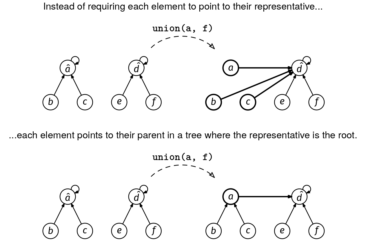
This can be generalized to multiple layers of indirection. To find an element's representative, we keep following parent pointers until we find an element that points to itself. That is the representative.

The resulting structure looks like a forest with one rooted tree for each group, with the representative as the root.

Now, we can union two groups by moving a single pointer in constant time (however, this version is still not the definitive one):

# Version without optimizations -- Do not use in interviews.
class UnionFind:
    def __init__(self):
        self.parent = dict()

    def add(self, x):
        self.parent[x] = x

    def find(self, x):
        root = self.parent[x]
        while self.parent[root] != root:
            root = self.parent[root]
        return root

    def union(self, x, y):
        repr_x, repr_y = self.find(x), self.find(y)
        if repr_x == repr_y:
            return  # They are already in the same set.
        self.parent[repr_x] = repr_y

In this forest-based implementation, the find() method iteratively traverses parents in the tree until it reaches the root. When it comes to trees, the worst case is always when the tree is as unbalanced as possible. This implementation does not work well in the worst case because we could end up with a long chain of parents, slowing down the finding of representatives for elements deep in the chain.

Luckily, we can make this forest approach very efficient by sprinkling in a couple of optimizations: path compression and union by size. The idea is that we want shallow trees without requiring us to update too many parent pointers.

Optimization 1: Path Compression

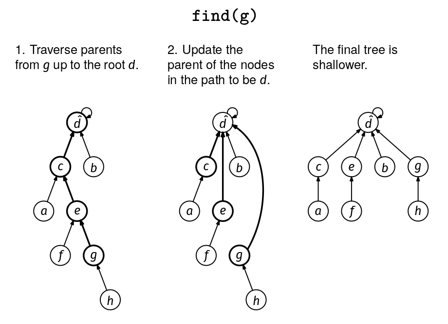
In the find(x) method, we need to traverse the chain of parents from x to the root of its tree. This takes O(d) time, where d is the depth of x in the tree. The path compression optimization is simple: once we find the root, we can update the parent of all the ancestors of x to point directly to the root. This way, if we call find() for any of them, we'll find the root in a single step. We implement this optimization by adding a second while loop in the find() method:

def find(self, x):
    root = self.parent[x]
    while self.parent[root] != root:
        root = self.parent[root]
    # Path compression optimization:
    while x != root:
        self.parent[x], x = root, self.parent[x]
    return root

The second while loop does the same number of iterations as the first one, so the path compression optimization does not change the worst-case complexity of find(x).

With just the path compression optimization, the union–find data structure is already very efficient: any sequence of n add(), union(), and find() operations takes O(n log n) time, meaning that each operation takes O(log n) amortized time (we omit the proof of this analysis, as it is not well known and thus not expected for you to know in an interview).

That is enough to pass any online assessment and probably enough to pass an in-person interview. So, consider this second optimization extra credit.

Optimization 2: Union by Size

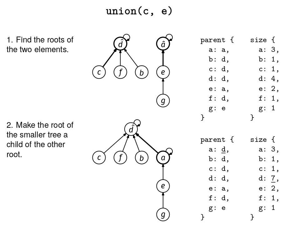
So far, when combining two groups, we did not care which group's representative became the new representative. As the name suggests, the "union by size" optimization is about being a bit smarter about this choice.¹ Let's say we need to merge two groups, A and B, and A has 5 elements while B has 100. If we make the root of A the parent of the root of B, then we increase the depth of 100 nodes. If we did the opposite, we would increase the depth of only 5 nodes. The latter is better!

To implement this, we need an additional map to keep track of the sizes of the groups:

class UnionFind:
    def __init__(self):
        self.parent = dict()
        self.size = dict()

    def add(self, x):
        self.parent[x] = x
        self.size[x] = 1

    def find(self, x):
        root = self.parent[x]
        while self.parent[root] != root:
            root = self.parent[root]
        while x != root:
            self.parent[x], x = root, self.parent[x]
        return root

    def union(self, x, y):
        repr_x, repr_y = self.find(x), self.find(y)
        if repr_x == repr_y:
            return  # They are already in the same set.
        if self.size[repr_x] < self.size[repr_y]:
            self.size[repr_y] += self.size[repr_x]
            self.parent[repr_x] = repr_y
        else:
            self.size[repr_x] += self.size[repr_y]
            self.parent[repr_y] = repr_x

The find() implementation does not change. In fact, the path compression and union by size implementation are independent, we can implement either without the other.

Note that we only care about the values in the size map for representatives, but we do not bother to remove elements from the size map when they are no longer representatives. We could do this to save some space, but it would not change the overall space analysis.

Advice for Implementing Union–Find in an Interview

Using union–find in an interview can be double the work: You might have to implement the data structure and use it to solve the problem. Our advice for in-person interview is:

1. Declare a class for your data structure with all the methods but without any implementation (like the API at the beginning of the chapter, but for your language).
2. Then, solve the problem using the class as if it was already implemented.
3. Finally, if you have time and the interviewer wants to see if you can implement the API (remember The Magic Question™ from the 'Anatomy of a Coding Interview' chapter), go back and fill in the missing implementation.

Doing it in this order ensures that you do not implement a data structure that later turns out not to be useful for your problem. It also ensures that you do part (2), which may get you partial credit even without (3).

In any case, you should be ready to implement the union–find data structure, as we usually see interviewers ask interviewees to implement it (unlike, e.g., heaps in JavaScript).

When you get to the union–find implementation phase of the interview, our recommendation is to start with the unoptimized forest-based implementation but with two comments at the top:

# TODO: path compression
# TODO: union by size

If you remember that (1) the data structure's name tells you its methods, and (2) the main internal data structure is the parent map, it should not be too hard to complete the unoptimized implementation even if you haven't memorized it.

The unoptimized implementation is enough to get a working solution. After getting the basics in place, you can use extra time to circle back and add the optimizations (especially the path compression one, which is easier).

Analysis

As mentioned, we get O(log n) amortized time per operation with just path compression. If we also add union by size, the time further improves to O(α(n)). The function α(n) is called the inverse Ackermann function,² and it is something we haven't seen before, as it never comes up outside of the union–find analysis. Without getting into its mathematical definition, all you need to know is that it grows even more slowly than the logarithm.
So slowly, in fact, that α(2^65536 - 3) = 4.

Applications

Graph Traversals vs Union–Find

The union–find data structure is closely related to the concept of connected components in undirected graphs. Imagine you have a graph and want to find the connected components. We can add all the nodes to a union–find data structure, and then call union(u, v) for each edge [u, v]. The final forest in the data structure will contain one tree for each connected component.

This idea was already present in the 'First Time All Connected' problem, where we added the cables connecting computers one by one until only a single group—or connected component—remained. In many problems about graph connectivity, we can use either a graph traversal solution—DFS or BFS—or a union–find solution. So, when should we use each?

Graph traversals are simpler to implement and marginally more efficient (O(V + E) vs O(E * α(V)), where V is the number of nodes and E is the number of edges), so they should be our go-to approach. However, there is one scenario where union–find is more powerful and makes more sense than graph traversals: when connections are added one at a time in a specific order (as in the 'First Time All Connected' problem). In problems like this, we care about the state of the graph (e.g., the number of connected components) after each step. It's like we have a sequence of incremental graphs instead of a single graph.

Minimum Spanning Tree

One of the classic applications of union–find is Kruskal's algorithm for the minimum spanning tree problem:

Given a weighted, undirected, connected graph, find a minimum spanning tree (MST) and return the sum of its edge weights.

• A spanning tree is a subset of edges that connects (i.e., "spans") every node and has no cycles.³
• The minimum spanning tree is the spanning tree with minimum edge weight sum.

The MST may not be unique.

The graph is given as an edge list. We are given V, the number of nodes, and edges, an edge list where each entry is a triplet [u, v, w], where u and v are the endpoints of an edge, and w is the weight. Nodes are identified by integers from 0 to V-1. Weights can be positive, zero, or negative.

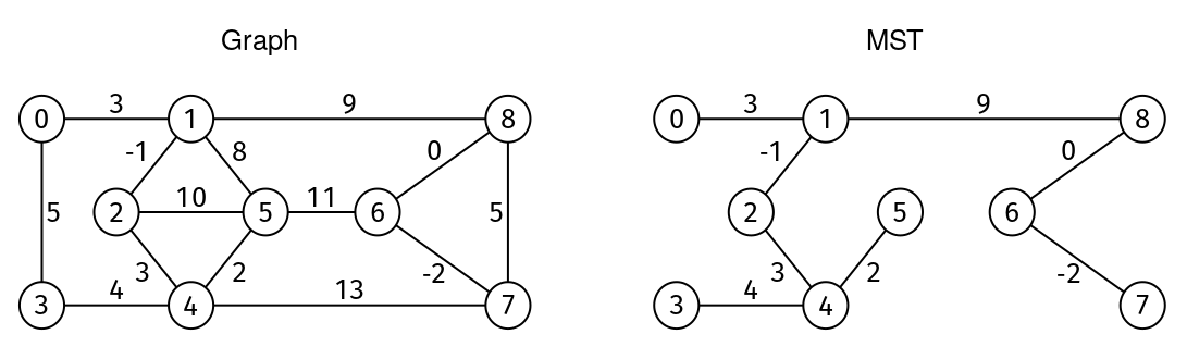
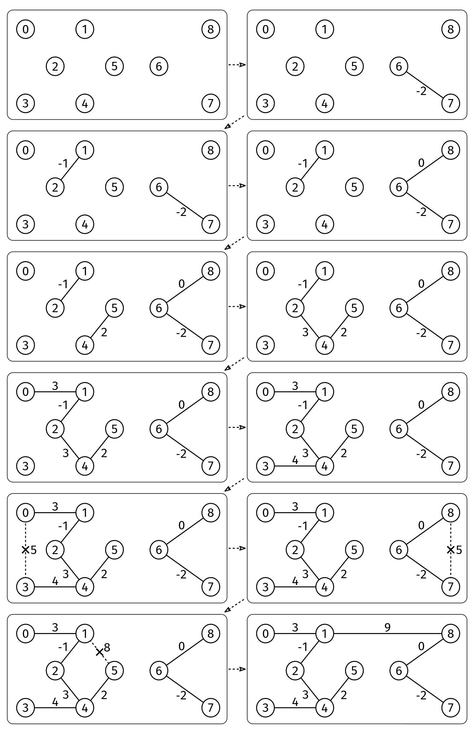
Example (see Figure 8):
V = 9
edges = [[0, 1, 3], [1, 8, 9], [8, 7, 5], [7, 4, 13], [4, 3, 4], [3, 0, 5], [1, 5, 8],
         [5, 4, 2], [4, 2, 3], [2, 1, -1], [2, 5, 10], [5, 6, 11], [6, 8, 0], [6, 7, -2]]

Output: 18
The sum of weights of MST edges is -2 + -1 + 0 + 2 + 3 + 3 + 4 + 9

There are multiple algorithms for this problem, like Prim's algorithm. Here, we will cover Kruskal's algorithm.

Kruskal's algorithm is a greedy algorithm that works as follows:

1. Order all the edges from smallest to largest weight.
2. Build the MST one edge at a time. Starting with an empty tree, for each edge in order, add it to the MST unless it creates a cycle.

Union–find is ideal for Kruskal's algorithm:

• We start with each node in its own connected component and connect them over time.
• For each edge, we need to know whether it makes a cycle, i.e., whether the endpoints are already in the same connected component. This type of cycle-detection question—or connectivity-related questions in general—is easy to answer with the union–find data structure: we just check if the two nodes have the same representative.
• It is important that we add the edges in a specific order, from smallest to largest (otherwise, we will get a spanning tree, but it may not be the minimum). This is our trigger for union–find as opposed to DFS or BFS.

def kruskal(V, edges):  # Assumes the graph is connected.
    uf = UnionFind()
    for u in range(V):
        uf.add(u)
    mst_cost = 0
    edges.sort(key=lambda edge: edge[2])
    for u, v, weight in edges:
        repr_u, repr_v = uf.find(u), uf.find(v)
        if repr_u != repr_v:
            uf.union(u, v)
            mst_cost += weight
    return mst_cost

The bottleneck of Kruskal's algorithm is sorting, which takes O(E log E) time, where E is the number of edges. The rest takes O(E * α(V)) time.

Problem Set

This problem set includes problems where the order of connections matters, so union–find is a great fit.

Add an operation, num_groups(), to the union–find data structure implementation that returns the current number of sets.

Follow-up: Simplify the solution to the 'First Time All Connected' problem we saw at the beginning of the chapter to use this operation instead.

Given a weighted, undirected graph, find a minimum spanning tree (MST) and return an array with the edges in it. If the MST is not unique, return any of them. If the graph is not connected, return an empty list.

Example 1:
V = 9
edges = [[0, 1, 3], [1, 8, 9], [8, 7, 5], [7, 4, 13], [4, 3, 4], [3, 0, 5], [1, 5, 8],
         [5, 4, 2], [4, 2, 3], [2, 1, -1], [2, 5, 10], [5, 6, 11], [6, 8, 0], [6, 7, -2]]
Output: [[0, 1, 3], [1, 8, 9], [4, 3, 4], [5, 4, 2], [4, 2, 3], [2, 1, -1], [6, 8, 0], [6, 7, -2]]
See Figure 8.

Example 2:
V = 3, edges = [[0, 1, 1]]
Output: []
The graph is not connected.

Example 3:
V = 3, edges = [[0, 1, 1], [1, 2, 1], [2, 0, 1]]
Output: [[0, 1, 1], [1, 2, 1]]
The solution is not unique.

Given a weighted, undirected graph, and an index i in the edge list, return whether the i-th edge must be part of the minimum spanning tree (meaning that any spanning tree that does not contain it has a higher cost than the MST).

Example 1:
V = 4, edges = [[0, 1, 5], [1, 2, 5], [2, 3, 20], [3, 0, 20]], i = 0
Output: True
The cost of the MST is 30. There are two MSTs with this cost, and both contain the edge [0, 1, 5]. Without it, the MST has cost 45.

Example 2:
V = 4, edges = [[0, 1, 5], [1, 2, 5], [2, 3, 20], [3, 0, 20]], i = 2
Output: False
There is an MST without the edge [2, 3, 20].

We are given an undirected graph as the number V of nodes and a list of edges where each edge is a triplet [u, v, time], where u and v are nodes between 0 and V - 1 (included) and time is a positive integer representing the time when the edge was added to the graph. We are also given a sorted list times with positive integers.

Return an array with the same length as times with the number of connected components at each time in times.

Example:
V = 4
edges = [[0, 1, 60], [0, 3, 180], [2, 3, 120]]
times = [30, 120, 210]
Output: [4, 2, 1]

At time 30, the graph has no edges yet, so each of the four nodes is its own connected component.
At time 120, the graph has edges (0, 1) and (2, 3), so it has two connected components.
At time 210, all nodes are in the same connected component.

The input is the same as Problem 5. Return an array with the same length as times with the size of the largest connected component at each time in times (instead of the number of connected components).

Example:
n = 4
edges = [[0, 1, 60], [0, 3, 180], [2, 3, 120]]
times = [30, 120, 210]
Output: [1, 2, 4]

A heated election has n parties. We are given two arrays of length n, candidates and votes, such that candidates[i] is the name of the candidate of the i-th party and votes[i] is the number of votes of the i-th party.

If a party has more than 50% of the votes, they win automatically. Otherwise, the following happens until a party wins: the two parties with the fewest votes create a coalition (if there is a tie, they all join the coalition): a new party with the votes of both and where the candidate is the candidate of the party that had more votes (breaking ties by the smallest alphabetical name of the candidate, which are unique). Return the name of the candidate that wins the election.

Example:
candidates = ["Ale", "Bloop", "Chip", "Dart", "Zing"]
votes = [10, 20, 30, 15, 25]
Output: Dart

Initially, no candidate has more than 50% of the votes (51 or more). Then, the parties of Ale and Dart form a coalition party with 25 votes and Dart as the representative. After that, Bloop's party has the fewest votes at 20, followed by Dart's and Zing's parties at 25. Therefore, the three form a new coalition party led by Dart (because Dart goes before Zing alphabetically). This new party has 70 votes, so it wins the election.

Problem set solutions.

We can do it in two ways:

1. Keep track of a num_ccs variable internally, increasing it when we call add() and decreasing it when we union two sets.
2. If we are using the union-by-size optimization: we delete size[u] from the size map whenever u stops being a representative (whenever we update the parent pointer of u to someone other than u). Then, the new function can simply return len(self.size).

We can adapt Kruskal's algorithm to the case where we do not know upfront if the graph is connected.

We can approach this problem in a few ways:

1. Of course, we could do a separate DFS just to check for connectivity at the beginning (but that is not in the spirit of the question!).
2. If we are using the union-by-size optimization, we can check in the size array if everyone is in the same group. We can add a check at the end:

if uf.size[uf.find(0)] != n:
    return -1

3. Without relying on the size array, we could instead keep track of the number of edges that we added to the MST and then check at the end if we added n-1 (recall that we need at least n-1 edges to connect n nodes).

Here is approach 3:

def kruskal(V, edges):
    uf = UnionFind()
    for u in range(V):
        uf.add(u)
    mst_edges = []
    edges.sort(key=lambda edge: edge[2])
    for u, v, weight in edges:
        repr_u, repr_v = uf.find(u), uf.find(v)
        if repr_u != repr_v:
            uf.union(u, v)
            mst_edges.append([u, v, weight])
            if len(mst_edges) == V - 1:
                return mst_edges
    return []  # The graph was not connected.

We can leverage Kruskal's algorithm to answer this question. We run it twice: once to find the real cost of the MST, and once to find the cost of the MST without the i-th edge.

def edge_in_mst(V, edges, i):
    mst_cost = kruskal(V, edges)
    mst_cost_without_i = kruskal(V, edges[:i] + edges[i+1:])
    return mst_cost != mst_cost_without_i

We can use a union–find data structure to track how the connected components evolve over time. We can sort the edges by the time they are added to the graph and use the union() method on the endpoints in that order. We can maintain a variable num_ccs that increases whenever the endpoints of an edge have different representatives.

As we add edges to the graph, we also need to match the times of the edges with the times in times. We can use a two-pointer approach, where one pointer iterates over the edges sorted by time and the other over the times.

def num_ccs_at_times(n, edges, times):
    edges.sort(key=lambda edge: edge[2])
    uf = UnionFind()
    for u in range(n):
        uf.add(u)
    num_ccs = n
    times_i = 0
    res = [0 for _ in range(len(times))]
    for u, v, time in edges:
        while times_i < len(times) and time > times[times_i]:
            res[times_i] = num_ccs
            times_i += 1
        repr_u, repr_v = uf.find(u), uf.find(v)
        if repr_u == repr_v:
            continue
        uf.union(u, v)
        num_ccs -= 1
    while times_i < len(times):
        res[times_i] = num_ccs
        times_i += 1
    return res

We can follow the same approach as Problem 4 but keep track of a variable max_cc with the size of the largest connected component based on the size array from the union by size optimization.

def max_cc_at_times(n, edges, times):
    edges.sort(key=lambda edge: edge[2])
    uf = UnionFind()
    for u in range(n):
        uf.add(u)
    max_cc = 1
    times_i = 0
    res = [0 for _ in range(len(times))]
    for u, v, time in edges:
        while times_i < len(times) and time > times[times_i]:
            res[times_i] = max_cc
            times_i += 1
        repr_u, repr_v = uf.find(u), uf.find(v)
        if repr_u == repr_v:
            continue
        uf.union(u, v)
        max_cc = max(max_cc, uf.size[uf.find(u)])
    while times_i < len(times):
        res[times_i] = max_cc
        times_i += 1
    return res

This problem is a bit of a misdirection. It seems like a good fit for union–find because we have a dynamic where "things" (in this case, political parties) get merged in a specific order. We could use the union method to simulate parties forming coalitions, and the concept of representatives maps well to the party candidates.

However, if we pay attention to how we choose which sets are joined together, union–find starts to seem less of a good fit. We have to union the two parties with the fewest votes, and union–find does not offer an easy way to track the sets with the fewest combined votes as merges happen. There is another data structure that is good for this use case: a min-heap.

In this implementation, we use the Heap API we defined in the Heaps chapter.

def winner(candidates, votes):
    total_votes = sum(votes)
    min_heap = Heap(higher_priority=lambda x, y: x[1] < y[1] or (x[1] == y[1] and x[0] < y[0]))
    for i in range(len(candidates)):
        if votes[i] > total_votes/2:
            return candidates[i]
        min_heap.push((candidates[i], votes[i]))

    while True:
        _, min_votes = min_heap.pop()
        cand, second_min_votes = min_heap.pop()
        votes = min_votes + second_min_votes
        while min_heap.size() > 0 and min_heap.top()[1] == second_min_votes:
            cand = min(new_cand, min_heap.top()[0])
            votes += min_heap.top()[1]
            min_heap.pop()
        if new_votes > total_votes/2:
            return new_cand
        min_heap.push((new_cand, new_votes))

Key Takeaways

When it comes to the union–find data structure, you should be ready to implement it in an interview—see the 'Advice for Implementing Union–Find in an Interview' section.

If you can do that, using it is usually straightforward—you just need to be aware of the triggers for when it is useful. Don't forget about its unique big O analysis.

Footnotes

1. There is another well known strategy, "union by rank," which achieves the same time complexity, so there is no need to learn both. ↩

2. The name "inverse Ackermann function" comes from the fact that it is the mathematical inverse of the Ackermann function. The Ackermann function grows very rapidly—faster than exponential or factorial functions—which is why its inverse grows so slowly. ↩

3. We talked about spanning trees in Problem 4: Spanning Tree in the Graphs chapter. ↩