Prerequisites: Dynamic Arrays, Sets & Maps. It is recommended to review those chapters from BCtCI before reading this one.

Introduction

We saw how to use sets and maps in the 'Sets & Maps' chapter (bctci.co/sets-and-maps). We saw that they often come in handy in coding interviews, and we discussed how to use them effectively.

Sets and maps are implemented in two main ways:

• Using hash tables.
• Using self-balancing binary search trees.

We can distinguish between the implementations by calling one HashSet and HashMap and the other TreeSet and TreeMap. They have different use cases in advanced scenarios, but for the basic APIs we'll define, the hash-table-based implementations are more common, as they have better asymptotic runtimes and are faster in practice.

Most programming languages provide built-in hash sets and hash maps. In this chapter, we will look at how they are implemented. This will allow us to learn about the important concepts of hashing and hash tables. See the 'Self-Balancing BSTs' section in the Trees chapter for a discussion on tree-based implementations.

We'll start with sets, which are a bit simpler than maps.

Hash Set Implementation

The set API is simple:

add(x):      if x is not in the set, adds x to the set
remove(x):   if x is in the set, removes it from the set
contains(x): returns whether the element x is in the set
size():      returns the number of elements in the set

A question for the reader: Why do sets not have a function like set(i, x), which sets an element at a particular index?¹

We will build upon the concepts of dynamic arrays from the 'Dynamic Arrays' chapter (see bctci.co/implement-dynamic-array) to show how to implement sets very efficiently, which is what makes sets a versatile data structure for coding interviews.

Naive Set Implementation

Let's start with a naive implementation idea and then identify its weaknesses so we can improve it—like we often do in interviews. What if we simply store all the set elements in a dynamic array? The issue with this idea is that checking if an element is in the set would require a linear scan, so the contains() method would not be very efficient.

By comparison, dynamic arrays do lookups by index, which means that we can jump directly to the correct memory address based on the given index. We would like to be able to do something similar for sets, where, just from an element x, we can easily find where we put it in the dynamic array.

Here is a promising idea in this direction, though still unpolished. Say you have a set of integers. Instead of putting all the elements in a single dynamic array, initialize your set data structure with, say, 1000 dynamic arrays, and then store each integer x in the array at index x % 1000. In this way, we no longer need to scan through a list of every element each time: if the user calls contains(1992), we only need to check the array at index 1992 % 1000 = 992. That is, we only need to scan through integers that have the same remainder when divided by 1000.

This crude idea could work well in certain situations, but it has two critical shortcomings that we still have to address.

• The first shortcoming has to do with the distribution of the integers in the set. Consider a situation where someone uses a set to store file sizes in bytes, and in their particular application all the file sizes happened to be in whole kilobytes. Every element stored in the set, like 1000, 2000, or 8000, would end up in the array at index 0. If all the elements end up in the same index, we are back at the starting point, having to do linear scans through all the elements.
• The second shortcoming is that even if the elements were perfectly distributed among the 1000 arrays, fixing the number of arrays to 1000 is too rigid. It might be overkill if we have only a few elements, and it might not be enough if we store a really large number of them.

In the next section, we will use hash functions to address the first shortcoming. For the second shortcoming, we will see a familiar technique from dynamic arrays: dynamic resizing.

Hash Functions

A hash function is a function that maps inputs of some type, such as numbers or strings, into a "random-looking" number in a predetermined output range. For instance, if h(x) is a hash function for integers with an output range of 0 to 999, then it could map 1 to 111, 2 to 832, and 3 to itself. Even though the mapping seems "random," it is important that each input always maps to the same value. That is, h(1) must always be 111. We say that 111 is the hash of 1.

In an actual hash function implementation, hashes are not truly random, but we want them to be "random-looking" because we consider a hash function good if it spreads the input values evenly across the output range, even if the distribution of input values is skewed in some way or follows some non-random pattern. For instance, h(x) = x % 1000 is not a good hash function because, even though each number from 0 to 999 is the hash of the same fraction of input values, we saw that we could get a very uneven distribution for certain input patterns—like if every input was a multiple of 1000. The challenge, then, is to spread the inputs evenly for any input pattern.

A simple hash function for integers

There are many interesting ways to hash integers into a fixed range such as [0, 999]. In this section, we will show a simple one known as multiplicative hashing. It may not have the best distribution properties, but it suffices to understand the concept and it runs in constant time.

We'll use m to denote the upper bound of the output range, which is excluded. In our example, m = 1000. Our hash function is based on the following observation: if we multiply an input integer by a constant between 0 and 1 with "random-looking" decimals such as 0.6180339887, we get a number with a "random-looking" fractional part. For instance,

• 1 * 0.618... = 0.618...
• 2 * 0.618... = 1.236...
• 3 * 0.618... = 1.854...

We can then take the fractional part alone, which is between 0 and 1, and multiply it by m to scale it up to the range between 0 and m. Finally, we can truncate the decimal part and output the integer part of this number, which will be a "random-looking" number between 0 and m-1.²

C = 0.6180339887   # A "random-looking" fraction between 0 and 1.

def h(x, m):
    x *= C         # A product with "random-looking" decimals.
    x -= int(x)    # Keep only the fractional part.
    x *= m         # Scale the number in [0, 1) up to [0, m).
    return int(x)  # Return the integer part.

When m = 1000, the function amounts to returning the first 3 decimals of x * C as our output hash between 000 and 999. For example:

• h(1, 1000) = 618 because 1 * 0.618... = 0.618...
• h(2, 1000) = 236 because 2 * 0.618... = 1.236...
• h(1000, 1000) = 33 because 1000 * 0.618... = 618.033...

There will be cases where different inputs have the same hash. Those are called collisions. For instance, 2 collides with 612:

• h(612, 1000) = 236 because 612 * 0.618... = 378.236...

If the number of possible inputs is larger than the output range, collisions are unavoidable.³

Hash functions in sets

If you think about it, in our naive set implementation, we used a sort of hash function to map inputs to one of our 1000 dynamic arrays: h(x, 1000) = x % 1000. However, as we saw, this hash function could result in a ton of collisions for certain input patterns. If we had used multiplicative hashing instead, we would have distributed the inputs much better. We'll see how it all comes together at the end of the section.

Hashing strings

We want to be able to hash different types, not just integers. Strings are a type we often need to hash, but this poses the extra challenge of different input and output types: string -> number.

We'll follow a two-step approach:

1. Convert the string into a number,
2. Once we have a number, use the modulo operator (%) to get a remainder that fits in the output range. For instance, if the output range is 0 to 999, we would set m = 1000 and do:

def h(str, m):
    num = str_to_num(str)
    return num % m

In Step (2), we could apply integer hashing (like multiplicative hashing) to the number returned in Step (1), but if the numbers returned by Step (1) are unique enough, the modulo operation is usually enough.

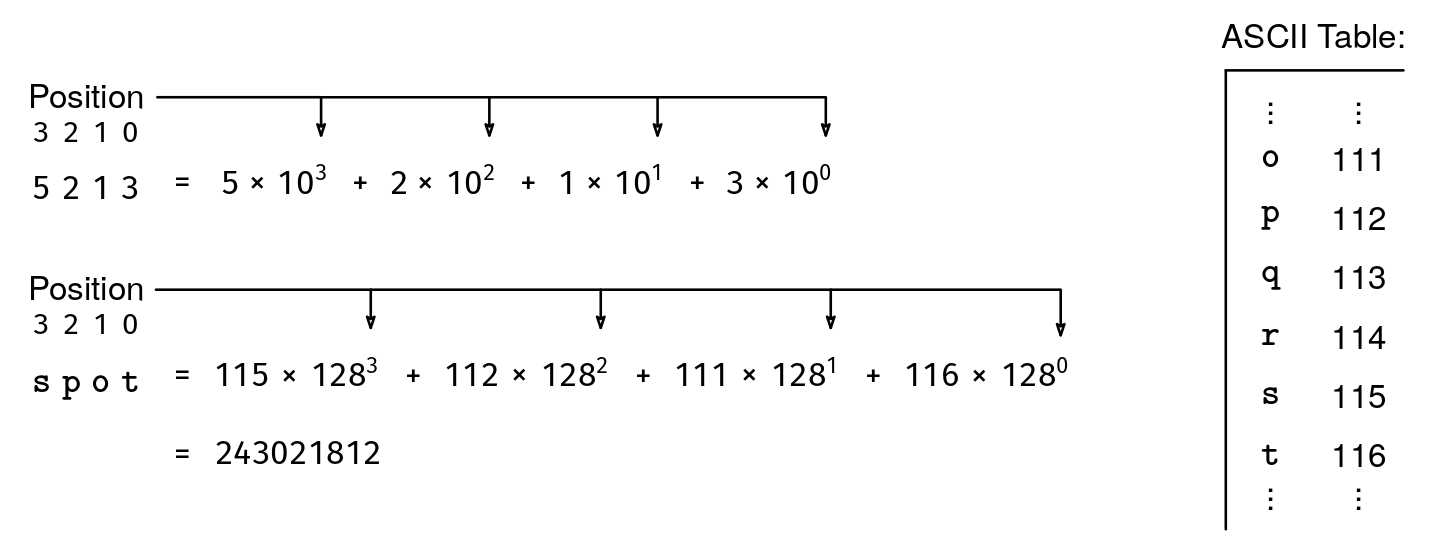
So, how can we convert strings into numbers? Since characters are encoded in binary, we can treat each character as a number. For instance, in Python, ord(c) returns the numerical code of character c. For this section, we will assume that we are dealing with ASCII strings, where the most common characters, like letters, numbers, and symbols, are encoded as 7-bit strings (numbers from 0 to 127).⁴

Can we use ASCII codes of the individual characters to convert a whole string into a single number?

Problem set. Each of the following proposed implementations for the str_to_num() method, which converts strings to integers, is not ideal. Do you see why? Can you identify which input strings will result in collisions (the same output number)?

1. Return the ASCII code of the first character in the string.
2. Return the ASCII code of the first character in the string multiplied by the length of the string.
3. Return the sum of the ASCII code of each character.
4. Return the sum of the ASCII code of each character multiplied by the character's index in the string (starting from 1).

Solution.

1. This function is bad because any two strings starting with the same character, like "Mroczka" and "McDowell", end up with the same number: ASCII(M) = 77. Another way to see that it is bad is that it can only output 128 possible different values, which is too small to avoid collisions.
2. This function is less bad because, at least, it can output a much larger set of numbers. However, there can still be many collisions. Any two strings starting with the same character and with the same length get the same number, like "aa" and "az": 97 * 2 = 194.
3. This function is much better because it factors in information from all the characters. Its weakness is that the order of the characters does not matter: the string "spot" maps to the number 115 + 112 + 111 + 116 = 454, but so do other words like "stop", "pots", and "tops".
4. This function is even better and results in fewer collisions because it uses information from all the characters and also uses the order. However, it is still possible to find collisions, like "!!" and "c". The ASCII code for '!' is 33, so the number for "!!" is 33 * 1 + 33 * 2 = 99, and the ASCII code for 'c' is also 99.

It turns out that there is a way to map ASCII strings to numbers without ever having any collisions. The key is to think of the whole string as a number where each character is a 'digit' in base 128 (see Figure 2). For instance, "a" corresponds to the number 97 because that's the ASCII code for 'a', and "aa" corresponds to 12513 because (97 * 128^1) + (97 * 128^0) = 12513.

def str_to_num(str):
    res = 0
    for c in str:
        res = res * 128 + ord(c)
    return res

The cost to pay for having unique numbers is that we quickly reach huge numbers, as shown in Figure 2. In fact, the numbers could easily result in overflow when using 32-bit or 64-bit integers (128^10 > 2^64, so any string of length 11 or more would definitely overflow with 64-bit integers).

To prevent this, we add a modulo operation to keep numbers in a manageable range. For instance, if we want the number to fit within a 32-bit integer, we can divide our number by a large prime that fits in 32 bits like 10^9 + 7 and keep only the remainder.⁵

LARGE_PRIME = 10**9 + 7

def str_to_num(str):
    res = 0
    for c in str:
        res = (res * 128 + ord(c)) % LARGE_PRIME
    return res

We want LARGE_PRIME to be large to maximize the range of possible remainders and have fewer collisions. We want it to be prime because non-prime numbers can lead to more collisions for specific input distributions. For instance, when dividing numbers by 12, which has 3 as a factor, every multiple of 3 has a remainder of 0, 3, 6, or 9. That means that if our input distribution consisted of only multiples of 3, we would have a lot of collisions. Prime numbers like 11 do not have this issue except for multiples of 11 itself.⁶

This is a good way to map strings into integers without overflowing. The runtime is proportional to the string's length. In the 'Rolling Hash Algorithm' section, we will see another application of this method.

Putting it All Together

Implement a hash set which supports add(), contains(), remove(), and size().

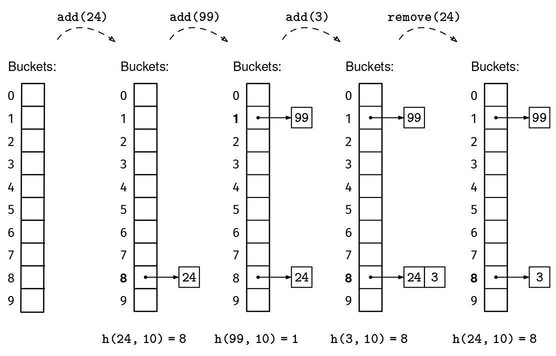
Our final set implementation will consist of a dynamic array of buckets, each bucket being itself a dynamic array of elements.⁷ The outer array is called a hash table. The number of elements is called the size, and the number of buckets is called the capacity. We can start with a modest capacity, like 10:

class HashSet:
    def __init__(self):
        self.capacity = 10
        self._size = 0
        self.buckets = [[] for _ in range(self.capacity)]

    def size(self):
        return self._size

In this context, size has the same meaning as for dynamic arrays, but capacity is used a bit differently, since all buckets can be used from the beginning. We use a hash function h() to determine in which bucket to put elements: element x goes in the bucket at index h(x, m), where m is the number of buckets in the hash table (the capacity).⁸ The specific hash function will depend on the type of the elements, but using a good hash function will guarantee that the buckets' lengths are well-balanced.

def contains(self, x):
    hash = h(x, self.capacity)
    for elem in self.buckets[hash]:
        if elem == x:
            return True
    return False

The final piece to complete our set data structure involves how to dynamically adjust the number of buckets based on the number of elements in the set. On the one hand, we do not want to waste space by having a lot of empty buckets. On the other hand, in order for lookups to take constant time, each bucket should contain at most a constant number of elements. The size/capacity ratio is called the load factor. In other words, the load factor is the average length of the buckets.

A good load factor to aim for is 1. That means that, on average, each bucket contains one element. Of course, some buckets will be longer than others, depending on how lucky we get with collisions, which are unavoidable. But, if the hash function manages to map elements to buckets approximately uniformly, with a load factor of 1 the expected longest bucket length is still constant.

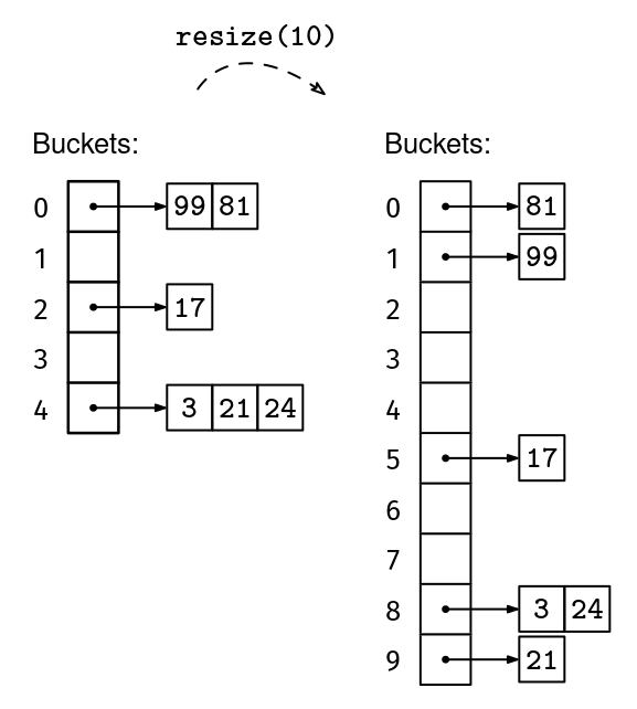
Remember how, with dynamic arrays, we had to resize the fixed-size array whenever we reached full capacity? With hash tables, we will do the same: we will relocate all the elements to a hash table twice as big whenever we reach a load factor of 1.⁹ The only complication is that when we move the elements to the new hash table, we will have to re-hash them because the output range of the hash function will have also changed. We now have all the pieces for a full set implementation.

def add(self, x):
    hash = h(x, self.capacity)
    for elem in self.buckets[hash]:
        if elem == x:
            return
    self.buckets[hash].append(x)
    self._size += 1
    load_factor = self._size / self.capacity
    if load_factor > 1:
        self.resize(self.capacity * 2)

def resize(self, new_capacity):
    new_buckets = [[] for _ in range(new_capacity)]
    for bucket in self.buckets:
        for elem in bucket:
            hash = h(elem, new_capacity)
            new_buckets[hash].append(elem)
    self.buckets = new_buckets
    self.capacity = new_capacity

Finally, when removing elements from the set, we downsize the number of buckets if the load factor becomes too small, similar to how we did for dynamic arrays. We can halve the number if the load factor drops below 25%.

def remove(self, x):
    hash = h(x, self.capacity)
    for i, elem in enumerate(self.buckets[hash]):
        if elem == x:
            self.buckets[hash].pop(i)
            self._size -= 1
            load_factor = self._size / self.capacity
            if load_factor < 0.25 and self.capacity > 10:
                self.resize(self.capacity // 2)

This completes our set implementation.

Hash Set Analysis

The contains() method has to compute the hash of the input and then loop through the elements hashed to a particular bucket. Assuming we have a decent hash function and a reasonable load factor, we expect each slot to be empty or contain very few elements. Thus, the expected runtime for a set of integers is O(1). It is worth mentioning that this expectation only applies with a high-quality hash function!

The add() method has the same amortized analysis as our dynamic array. Most additions take O(1) expected time, since we just find the correct bucket and append the value to it. We occasionally need to resize the array, which takes linear time, but, like with dynamic arrays, this happens so infrequently that the amortized runtime per addition over a sequence of additions is still O(1). The analysis for remove() is similar.

Thus, we can expect all the set operations to take constant time or amortized constant time. If the elements are strings, we also need to factor in that hashing a string takes time proportional to the size of the string. One simple way to phrase this is that we can expect the operations to take O(k) amortized time, where k is the maximum length of any string added to the set.

Hash Set Problem Set

The following problem set asks data structure design questions related to hash sets.

Add the following methods to our HashSet class. For each method, provide the time and space analysis.

1. Implement an elements() method that takes no input and returns all the elements in the set in a dynamic array.
2. Implement a union(s) method that takes another set, s, as input and returns a new set that includes all the elements in either set. Do not modify either set.
3. Implement an intersection(s) method that takes another set as input, s, and returns a new set that includes only the elements contained in both sets. If the sets have no elements in common, return an empty set. Do not modify either set.

A multiset is a set that allows multiple copies of the same element. Implement a Multiset class with the following methods:

add(x):      adds a copy of x to the multiset
remove(x):   removes a copy of x from the multiset
contains(x): returns whether x is in the multiset (at least one copy)
size():      returns the number of elements in the multiset (including copies)

Problem set solutions.

1. elements(): We can start by initializing an empty dynamic array. Then, we can iterate through the list of buckets, and append to the list all the elements in each bucket. The runtime is O(capacity + size) = O(size) (since the load factor is at least 25%, so the capacity is at most four times the size), and the space complexity is O(size).
2. union(s): We can start by initializing an empty set. Then, we can iterate through the elements in both self and s and call add(x) on the new set for each element x.
3. intersection(s): We can start by initializing an empty set. Then, we can iterate through the elements in self and call add(x) on the new set only for those elements where s.contains(x) is true.

We can approach it in two ways:

1. We can tweak the HashSet implementation we already discussed. The contains(), remove(), and size() methods do not change. For add(), we need to remove the check for whether the element already exists.
2. Alternatively, we could implement the multiset as a hash map with the elements in the set as keys and their counts as values.

Approach 2 is more common because it can save space: if we add n strings of length k, we'll use only O(k) space instead of O(n * k) for Approach 1. See the next section for more on maps.

Hash Map Implementation

As we have seen, sets allow us to store unique elements and provide constant time lookups (technically, it is amortized constant time, and only with a good hash function). Maps are similar, but the elements in a map are called keys, and each key has an associated value. Like elements in sets, map keys cannot have duplicates, but two keys can have the same value. The type of values can range from basic types like booleans, numbers, or strings to more complex types like lists, sets, or maps.

Map API:

add(k, v):   if k is not in the map, adds key k to the map with value v
             if k is already in the map, updates its value to v

remove(k):   if k is in the map, removes it from the map

contains(k): returns whether the key k is in the map

get(k):      returns the value for key k
             if k is not in the map, returns a null value

size():      returns the number of keys in the map

For instance, we could have a map with employee IDs as keys and their roles as values. This would allow us to quickly retrieve an employee's role from their ID.

Thankfully, we do not need to invent a new data structure for maps. Instead, we reuse our HashSet implementation and only change what we store in the buckets. Instead of just storing a list of elements, we store a list of key–value pairs. As a result, maps achieve amortized constant time for all the operations like sets.

We will leave the details of map internals as our final problem set in this chapter. In particular, you can find the full HashMap implementation in the solution to Problem 4 (bctci.co/hash-map-class).

Hash Map Problem Set

The following problem set asks data structure design questions related to maps.

Implement a HashMap class with the API described in the 'Hash Map Implementation' section.

Hint: you can modify the existing HashSet class to store key–value pairs.

Provide the time and space analysis of each method.

1. Implement a keys() method that takes no input and returns a list of all keys in the map. The output order doesn't matter.
2. Implement a values() method that takes no input and returns a list of the values of all the keys in the map. The output order doesn't matter. If a value appears more than once, return it as many times as it occurs.

A multimap is a map that allows multiple key–value pairs with the same key. Implement a Multiset class with the following methods:

add(k, v):   adds key k with value v to the multimap, even if key k is already found

remove(k):   removes all key-value pairs with k as the key

contains(k): returns whether the multimap contains any key-value pair with k as the key

get(k):      returns all values associated to key k in a list
             if there is none, returns an empty list

size():      returns the number of key-value pairs in the multiset

Problem set solutions.

We can adapt the HashSet class. The main difference is that, in add(), we need to consider the case where the key already exists, and we just update its value.

This was the add() method for the HashSet class:

def add(self, x):
    hash = h(x, self.capacity)
    for elem in self.buckets[hash]:
        if elem == x:
            return
    self.buckets[hash].append(x)
    self._size += 1
    load_factor = self._size / self.capacity
    if load_factor > 1:
        self.resize(self.capacity * 2)

And this is the modified version for the HashMap class:

def add(self, k, v):
    hash = h(k, self.capacity)
    for i, (key, _) in enumerate(self.buckets[hash]):
        if key == k:
            self.buckets[hash][i] = (k, v)
            return
    self.buckets[hash].append((k, v))
    self._size += 1
    load_factor = self._size / self.capacity
    if load_factor > 1:
        self.resize(self.capacity * 2)

The get() method is very similar to contains().

1. keys(): This is analogous to the elements() method from the Set Quiz.
2. values(): This is like keys(), but getting the values instead.

A multimap with values of type T can be implemented as a map where the values are arrays of elements of type T. The add() method appends to the array, the get() method returns the array, and remove() works as usual.

Rolling Hash Algorithm

Before wrapping up the chapter, we will illustrate a clever application of hash functions outside of hash sets and maps. Recall 'Problem 3: String Matching' from the String Manipulation chapter (bctci.co/string-matching):

Implement an index_of(s, t) method, which returns the first index where string t appears in string s, or -1 if s does not contain t.

A naive approach would be to compare t against every substring of s of the same length as t. If sn and tn are the lengths of s and t, there are sn - tn + 1 substrings of s of length tn. Comparing two strings of length tn takes O(tn) time, so in total, this would take O((sn - tn + 1) * tn) = O(sn * tn) time.

We can do better than this naive algorithm. The Knuth-Morris-Pratt (KMP) algorithm is a famous but tricky algorithm for this problem that runs in O(sn) time, which is optimal. Here, we will introduce the rolling hash algorithm, another famous algorithm that is also optimal and which we find easier to learn and replicate in interviews.

The basic idea is to compare string hashes instead of strings directly. For instance, if s is "cbaabaa" and t is "abba", we compare h("abba") with h("cbaa"), h("baab"), h("aaba"), and h("abaa"). If no hashes match, we can conclusively say that t does not appear in s. If we have a match, it could be a collision, so we need to verify the match with a regular string comparison. However, with a good hash function, 'false positives' like this are unlikely.

Since we are not actually mapping strings to buckets like in a hash table, we can use the str_to_num() function that we created in the 'Hashing strings' section as our hash function.

However, computing the hash of each substring of s of length tn would still take O(sn * tn) time, so this alone doesn't improve upon the naive solution. The key optimization is to compute a rolling hash: we use the hash of each substring of s to compute the hash of the next substring efficiently.

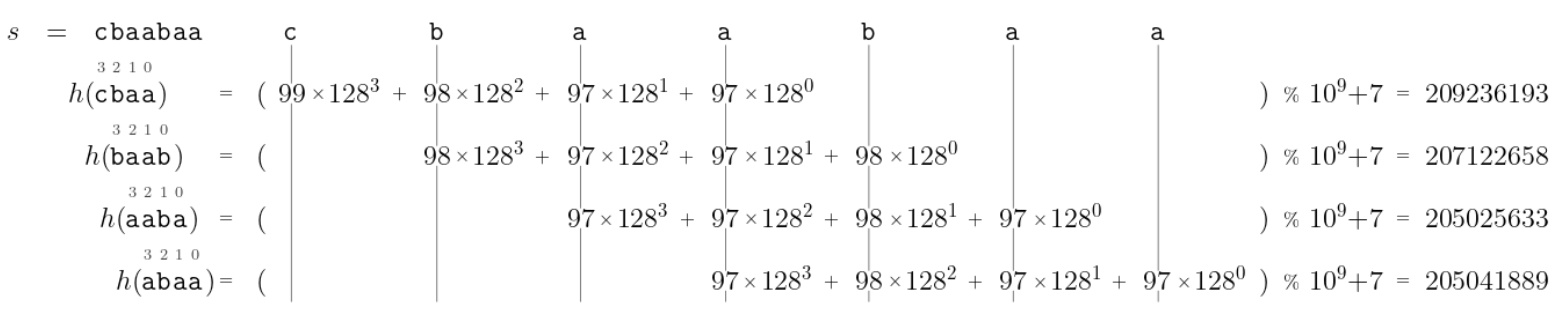
So, how can we go from, e.g., h("cbaa") to h("baab")? We can do it in three steps. Recall that ASCII('a') = 97, ASCII('b') = 98, and ASCII('c') = 99. We start with:

h("cbaa") = 99 * 128^3 + 98 * 128^2 + 97 * 128^1 + 97 * 128^0 = 209236193

Then:

1. First, we remove the contribution from the first letter, 'c', by subtracting 99 * 128^3. Now, we have:

98 * 128^2 + 97 * 128^1 + 97 * 128^0 = 1618145

2. Then, we multiply everything by 128, which effectively increases the exponent of the 128 in each term by one. This is kind of like shifting every letter to the left in Figure 5. Now, we have:

98 * 128^3 + 97 * 128^2 + 97 * 128^1 = 207122560

3. Finally, we add the contribution of the new letter, 'b', which is 98 * 128^0. We end up with:

98 * 128^3 + 97 * 128^2 + 97 * 128^1 + 98 * 128^0 = 207122658

This is h("baab"). We are done!

Here is a little function to do these steps. Note that we use modulo (%) at each step to always keep the values bounded within a reasonable range.¹⁰

# Assumes that current_hash is the hash of s[i:i+tn].
# Assumes that first_power is 128^(tn-1) % LARGE_PRIME.
# Returns the hash of the next substring of s of length tn: s[i+1:i+tn+1].
def next_hash(s, tn, i, current_hash, first_power):
    res = current_hash
    # 1. Remove the contribution from the first character (s[i]).
    res = (res - ord(s[i]) * first_power) % LARGE_PRIME
    # 2. Increase every exponent.
    res = (res * 128) % LARGE_PRIME
    # 3. Add the contribution from the new character (s[i+tn]).
    return (res + ord(s[i + tn])) % LARGE_PRIME

Each step takes constant time, so, from the hash of a substring of s, we can compute the hash of the next substring in constant time.

We pass 128^(tn-1) % 10^9 + 7 as the first_power parameter so that we do not need to compute it for each call to next_hash(), as that would increase the runtime. This way, we compute the hashes of all the substrings of length t in O(sn) time. Putting all the pieces together, we get the rolling hash algorithm:

LARGE_PRIME = 10**9 + 7

def power(x):
    res = 1
    for i in range(x):
        res = (res * 128) % LARGE_PRIME
    return res

def index_of(s, t):
    sn, tn = len(s), len(t)
    if tn > sn:
        return -1

    hash_t = str_to_num(t)
    current_hash = str_to_num(s[:tn])
    if hash_t == current_hash and t == s[:tn]:
        return 0  # Found t at the beginning.

    first_power = power(tn - 1)
    for i in range(sn - tn):
        current_hash = next_hash(s, tn, i, current_hash, first_power)
        if hash_t == current_hash and t == s[i + 1:i + tn + 1]:
            return i+1
    return -1

With a good hash function like the one we used, which makes collisions extremely unlikely, this algorithm takes O(sn) time, which is optimal.

This algorithm could also be called the sliding hash algorithm since it is an example of the sliding window technique that we learned about in the Sliding Window chapter (bctci.co/sliding-windows).

Key Takeaways

The following table should make it clear why hash sets and hash maps, as we built them in this chapter, are one of the first data structures to consider when we care about performance and big O analysis:

However, it is important to remember the caveats:

• The runtimes for add() and remove() are amortized because of the dynamic resizing technique, which can make a single add() or remove() slow from time to time.
• All the runtimes (except size()) are expected runtimes, and only when we are using a good hash function. In this chapter, we saw examples of good hash functions for integers and strings, and similar ideas can be used for other types.
• A common mistake is forgetting that hashing a string takes time proportional to the length of the string, so hash set and hash map operations do, in fact, not take constant time for non-constant length strings.

The 'Sets & Maps' chapter (bctci.co/sets-and-maps) shows how to make the most of these data structures in the interview setting.

Footnotes

1. Unlike arrays, sets do not have index-based setters and getters because elements are not in any particular order. ↩

2. A bad choice for the constant between 0 and 1 would be a simple fraction like 1/2, because then all even numbers would get hashed to 0 and all odd numbers would get hashed to m/2. Here, we are using the inverse of the golden ratio, φ = 1.618033... because it is the constant Donald Knuth used when he introduced this technique in his book The Art of Computer Programming. When using 1/φ as the constant, the hash function is known as "Knuth's multiplicate hashing," as well as "Fibonacci hashing" because of the relationship between the golden ratio and the fibonacci sequence. However, the exact constant used is not the point—you do not need to memorize any "magic constants" for your interviews. ↩

3. Mathematicians call this the "pigeonhole principle". If you think of the inputs as pigeons and the hashes as holes, it says that if there are more pigeons than holes, some pigeons (inputs) will have to share a hole (have the same hash). ↩

4. See the 'String Manipulation' Chapter in BCtCI for more on the ASCII format. ↩

5. Intermediate values may still exceed 32 bits, so, for typed languages, make sure to use 64-bit integers for the intermediate operations. ↩

6. There is nothing special about the number 10^9 + 7—it is just a large prime that fits in a 32-bit integer and is easy to remember because it is close to a power of ten. Any large prime would work well. Again, it is not important to memorize magic constants for interviews—you can always use a placeholder variable "LARGE_PRIME". ↩

7. Another popular data structure for each bucket is a linked list, which we learned about in the Linked Lists chapter (bctci.co/linked-lists). ↩

8. This strategy of handling collisions by putting all the colliding elements in a list is called separate chaining. There are other strategies, like linear probing or cuckoo hashing, but knowing one is probably enough. ↩

9. The exact load factor value is not important. Values slightly less or slightly more than one still have the same properties. Between a load factor of 0.5 and 1.5 there is a bit of a trade off between space and lookup time, but the asymptotic complexities don't change. ↩

10. Depending on the language, we have to be careful about Step 1 because the numerator (res - ord(s[i]) * first_power) can be negative. In Python, -7 % 5 = 3, which is what we want, but in other languages like JS, Java, and C++, -7 % 5 = -2, which is not what we want. We can fix it by adding LARGE_PRIME to the result, and applying % LARGE_PRIME once again. ↩