Double-Edge Cut Problem

In this post, we'll solve a graph problem that comes up in the Wall Game.

See also the related, but easier, Single-Edge Cut Problem.

The double-edge cut problem

You are given an undirected, unweighted graph G with V nodes and E edges, where each node is identified by an integer from 0 to V - 1. You are also given a pair of distinct nodes, s and t, in the same connected component of G.

We say a pair of edges (e1, e2) is essential if removing e1 and e2 from G disconnects s and t.

Implement a data structure that takes G, s, and t at construction time, and then can answer queries of the form "Is a given pair of edges essential?"

In this post, we'll see how to construct such a data structure in linear time and space (O(V + E)) and answer queries in constant time.

Example:

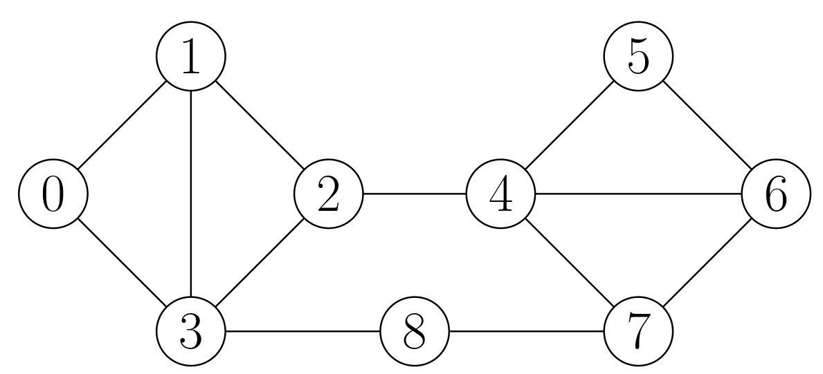
In this graph, if s is 0 and t is 6, the essential pairs are ((0, 1), (0, 3)), ((2, 4), (3, 8)), and ((2, 4), (7, 8)).

Any other pair of edges can be removed and s and t will remain in the same connected component, even if the graph itself is disconnected. For instance, if we remove (4, 5) and (5, 6), node 5 ends in its own connected component, but s and t are still connected.

Brute force solution

The brute force solution is to do nothing at construction time. For each query, take each pair of edges, remove them, and then use a graph traversal to see if s and t are still connected. This takes O(E) time per query.

The brute force implementation is on github. We'll compare it against the optimized solution in the benchmark at the end.

Motivation

This is the key problem behind whether a double-wall move is valid or not in the Wall Game. The board of the Wall Game may look something like the picture on the left:

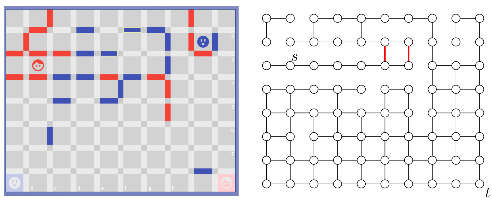
The right picture is the board modeled as a graph. The cells become nodes and two adjacent nodes are connected if there is no wall between them.

During their turn, players can build up to two walls anywhere, which is like removing two edges. The only constraint is that they cannot fully block the opponent's path to their goal (or their own). In this setting, each player forms an s-t pair with their goal, and the essential edge pairs correspond to invalid double-wall moves.

In the picture, the red player and goal are labeled s and t, and one essential pair is shown in red. There are many more essential pairs.

Imagine that you want to implement an engine for the Wall Game. One question you'll probably have to answer frequently is, "Given a position, is a given move valid?" The hardest type of move to check is a double wall move (the single-wall move case is handled by the single-edge cut problem). To answer this question efficiently, we can solve the double-edge cut problem and build one data structure for each player; we can query them to check if a double wall move disconnects any player from their goal.

Backstory

I got nerd-sniped by this problem in 2021, when I was coding an engine for the Wall Game (it's on github; it's in C++ but you can play against it on wallwars.net thanks to WebAssembly). The engine is based on negamax with alpha-beta pruning, and the bottleneck is generating all the valid double-wall moves from a position.

The move generation implementation from back then already uses some of the ideas we'll see in this post, like the fact that we can precompute two node-disjoint paths for each biconnected component, and two walls can only be an invalid if they are in the same biconnected component and there is one wall in each path (this will make sense later).

However, I couldn't figure out how to handle the case of two walls in the same biconnected component and in the two precomputed paths in constant time, defaulting to a full graph traversal for that case (here).

I revisited the problem in 2025 because I'm rebuilding the game. The key new insight is the construction of the path-segment graph, which we'll get to below. Something that was very helpful in this breakthrough was vibe coding a tool to visualize the various graph transformations (we'll see screenshots of it in this post).

Yes, I could have coded the visualization tool myself back then, but vibe coding removed the friction. Ironically, vibe coding has a rep for only being good at starting projects and then abandoning them, but here it helped me pick up an abandoned project and finish it.

Preliminary definitions

The algorithm relies heavily on the concepts of articulation points and biconnected components, so we'll need the following definitions:

• A biconnected graph is a graph that remains connected even if any single node is removed.
• An articulation point is a node whose removal increases the number of connected components. A graph is biconnected if and only if it has no articulation points.
• A biconnected component is a maximal biconnected subgraph.
• A bridge is an edge whose removal increases the number of connected components.

In a connected graph with at least two nodes, every node is in at least one biconnected component. The graph can be decomposed into what is called the block-cut tree of the graph, which has one node per biconnected component and biconnected components are connected by articulation points. For example:

This graph on the left has four articulation points: 2, 4, 6, and 7. It has six biconnected components (shown in different colors). The bridges are (7, 9), (7, 8), and (6, 12).

The block-cut tree is a tree in the sense that there cannot be a cycle of biconnected components--the cycle would collapse into a single biconnected component.

Here are some additional well known properties:

1. An articulation point is always in more than one biconnected component. For instance, node 7 in the picture above is in three biconnected components. An edge is always in a single biconnected component.
2. Not every edge between articulation points is a bridge. For instance, (2, 4) in the graph above is not a bridge.
3. Every node adjacent to a bridge is an articulation point with the exception of degree-1 nodes (like 9 in the picture above).
4. An edge is a bridge if and only if it is the only edge in a biconnected component.
5. In a biconnected component that is not a single edge, there are two node-disjoint paths between any two nodes. For instance, in the blue biconnected component, there are two paths from 2 to 4 that don't share any nodes: 2 -> 4 and 2 -> 10 -> 11 -> 4.
6. Two biconnected components can only have one articulation point in common. Otherwise, the two biconnected components would collapse into a single one.
7. There cannot be a cycle that is not fully contained in a single biconnected component. Otherwise, all the biconnected components in the cycle would collapse into a single one. (That's why the block-cut tree is called a tree.)
8. If a simple path (path with no repeated nodes) leaves a biconnected component, it cannot return to it (for similar reasons).

Reduction to biconnected graphs

In this section, we'll reduce the original problem to the case where the graph is biconnected, which we'll tackle in the next section.

Note that the graph from the Wall Game may not be biconnected. It may not even be connected--see, e.g., the isolated connected component in the top-left corner above. All we are guaranteed is that each player is in the same connected component as their goal.

First, we'll get an edge case out of the way: if s and t are neighbors and connected by a bridge, then an edge pair is essential if and only if it contains that bridge.

Next, consider the case where s and t are in the same biconnected component, C (which is not just a bridge). Any edge pair where at least one edge is in another biconnected component is not essential. Thus, we can focus on edge pairs inside C. In fact, when analyzing if an edge pair in C is essential, we can completely ignore the rest of the graph (we can literally remove nodes and edges outside of C). That is because any simple path from s to t must be fully contained in C (Property 8).

If s and t are not already in the same biconnected component, any path from s to t must go through the exact same sequence of articulation points and biconnected components. Otherwise, there would be a cycle of biconnected components, which is impossible (Property 7).

Let C1, C2, ..., Ck be the sequence of biconnected components that any s-t path must go through. In fact, not only is the sequence of biconnected components fixed, but also the entry and exit nodes of each biconnected component. The entry and exit nodes must be an articulation point, except for C1, where the entry node is s, and Ck, where the exit node is t. This is because there cannot be two articulation points from Ci to Ci+1 (Property 6).

Among the biconnected components between s and t, there may be one or more consisting of a single edge (i.e., a bridge). Removing that bridge disconnects s and t by itself, so any edge pair containing it is automatically essential.

Aside from the specific case of bridge-only biconnected components, there is no way to disconnect s and t by removing two edges from different biconnected components.

What that means is that we can tackle each biconnected component C1, C2, ..., Ck independently, and then combine the results.

We can start by finding the biconnected components of the graph and any s-t path. From there, we can decompose the input graph into C1, C2, ..., Ck, and solve the problem for each of them. Instead of s and t, for each biconnected component, we use the path's entry and exit nodes as the new s and t.

This all can be done in linear time, and allows us to reduce the general case to a number of instances of the biconnected case, all of which combined have an equal or smaller size than the original graph.

Next, we'll focus exclusively on the special case where the input graph is biconnected.

Biconnected graphs

In this section, we assume that G is biconnected.

One obstacle we'll need to overcome is that we cannot possibly store every essential pair in our data structure given the time and space constraints. The worst case for the number of essential pairs in a biconnected graph is about (V^2)/4, which happens when the graph forms a single cycle, and s and t are as far apart as possible in the cycle, with (V - 2)/2 edges between them on each side. In this case, each edge on one side of the cycle forms an essential pair with each edge on the other side of the cycle, for a total of ((V - 2)/2)^2 pairs. Since we want a data structure that takes O(V+E) space, we'll need to store some information that uses less space than the essential pairs themselves, but still allows us to answer queries in constant time.

Finding two node-disjoint paths

In the algorithm, we'll need to find two node-disjoint paths between s and t, which we know exist because the graph is biconnected.

The naive approach of finding a simple path, removing the nodes, and then looking for a second path doesn't work, like in this case:

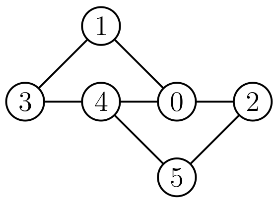
For example, in this graph, there are two node-disjoint paths from 3 to 2: 3 -> 1 -> 0 -> 2 and 3 -> 4 -> 5 -> 2. However, if we start by finding the path 3 -> 4 -> 0 -> 2 and remove nodes 4 and 0, we won't be able to find a second path.

Instead, we can use the following approach:

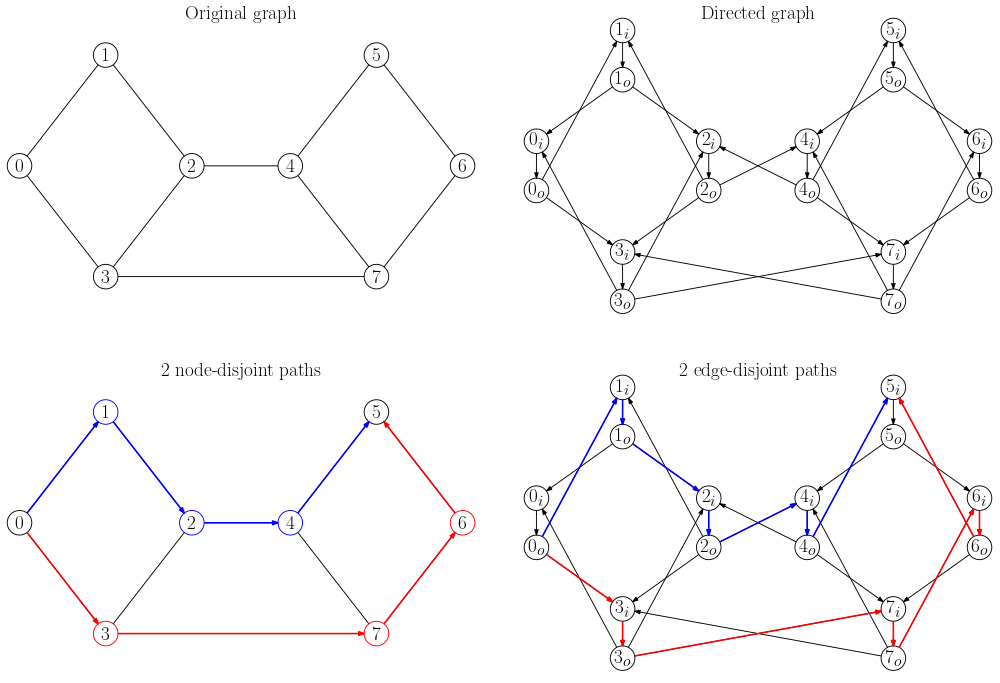
1. Take the undirected graph and convert it into a directed graph with the following transformation:

• Each node u becomes a pair of nodes, u_in and u_out, connected by an edge u_in -> u_out.
• Each undirected edge (u, v) becomes two directed edges, u_out -> v_in and v_out -> u_in. Note that the "out" nodes are always connected to "in" nodes. The only way to get to u_out is to come from u_in.

2. Next, we need to find two edge-disjoint paths from s_out to t_in in this directed graph. These two paths can be mapped to two node-disjoint paths in the original graph because, for each node u in the original graph, they can't both go through the edge u_in -> u_out in the directed graph.

This image shows a biconnected graph with two node-disjoint paths from 0 to 5:

Finding two edge-disjoint paths in a directed graph can be done with two iterations of the Ford-Fulkerson algorithm. Essentially, we can think of the directed graph as a flow network, where each edge has a capacity of 1. We then need to be able to send two units of flow from s to t. The paths of the flow form two edge-disjoint paths in the directed graph.

Building the directed graph takes linear time, and each iteration of Ford-Fulkerson algorithm requires a linear-time graph traversal. Thus, this all takes linear time (see the TypeScript implementation).

Essential edge candidates

Among all the edges in the biconnected graph, we will start by filtering down the edges that can be part of an essential pair to a smaller set of candidates.

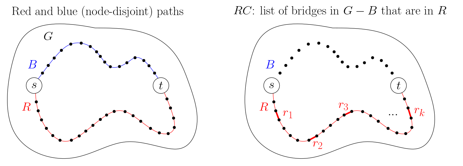
We start by finding any two node-disjoint paths from s to t, as described above. Which we'll call the red path (R) and the blue path (B). We'll call the edges in R red edges and the edges in B blue edges.

An edge pair can only be essential if it has one red edge and one blue edge (otherwise, s and t remain connected via one of the two paths). Thus, we can narrow down the set of candidate edges to those in R and B.

We can narrow the candidate edges further. Consider a red edge, e1. We know that if e1 is part of an essential pair, (e1, e2), then e2 must be a blue edge. So, if s and t remain connected even after removing e1 and all the blue edges, then we can safely say that e1 can never be part of an essential pair. That is, e1 is not a candidate.

We can find all the red candidates, which we'll call RC = (r1, r2, ..., rk), in linear time, as follows:

• Remove all the blue edges from G.
• Find all the bridges in the remaining graph.
• RC is the list of red bridges.

Similarly, we can find all the blue candidates, which we'll call BC = (b1, b2, ..., bk'), by removing all the red edges from G and finding the bridges in the remaining graph that overlap with B:

However, not every edge pair with one edge in RC and one edge in RB is essential. For example:

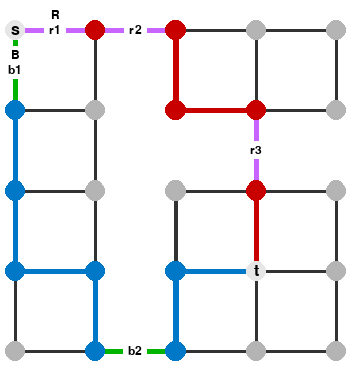
In this graph, the essential pairs are (r1, b1), (r2, b2), and (r3, b2). Other pairs of candidates, like (r1, b2), are not essential. Intuitively, a pair of candidates is not essential when we can stich together parts of the red and blue paths together that avoid the candidates.

The path-segment graph

We'll assume that RC and BC are both non-empty from now on (otherwise, we can just return False for every query).

To achieve worst-case constant-time queries, we'll need to construct what I call the path-segment graph:

This is an undirected graph that has one node for each disconnected segment of the red path after removing the red candidates, and one node for each disconnected segment of the blue path after removing the blue candidates.

In the path-segment graph, we call the nodes for the red segments rs_0, rs_1, ..., rs_k and the nodes for the blue segments bs_0, bs_1, ..., bs_k'. We'll also call them red-segment nodes and blue-segment nodes, respectively.

The nodes rs_0 and rs_1 are connected by an edge, which we call r1, just like in the original graph. Similarly, rs_1 and rs_2 are connected by r2, and so on, up to rs_k-1 and rs_k, which are connected by rk. The same applies to the blue-segment nodes, so every edge in RC and BC is "present" in the path-segment graph.

Besides the RC and BC edges, which connect the nodes of the red-segment nodes and blue-segment nodes in two separate paths, there are also cross edges between red-segment and blue-segment nodes. Intuitively, these edges denote that we can go from one segment of the red path to a segment of the blue path without crossing any of the candidate edges.

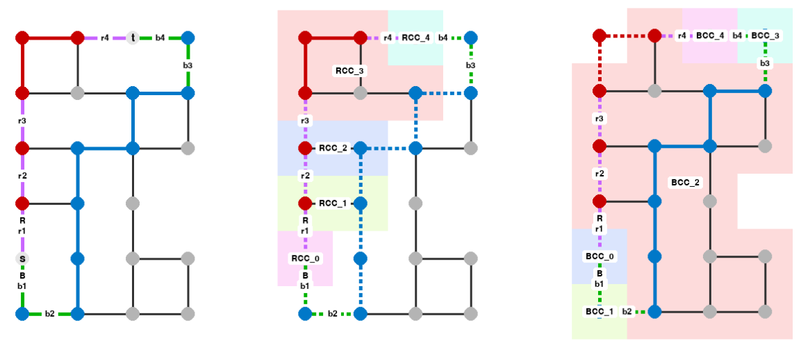
Here is the path-segment graph for the example above:

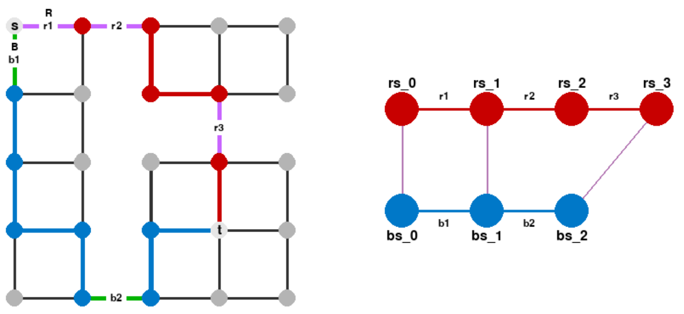
The red path is broken into four segments: rs_0 is just s, rs_1 is just the node between r1 and r2, rs_2 is the segment up to r3, and rs_3 is the final edge of the red path. Similarly, the blue path is broken into three segments.

In the path-segment graph, there is always a cross edge between rs_0 and bs_0 because they share the node s. Similarly, there is always a cross edge between rs_k and bs_k' because they share the node t. For this specific example, there is also a cross edge between rs_1 and bs_1 because we can walk from the node to the right of s to the segment of B that starts at the node below s without crossing any of the candidate edges.

Next, we'll describe how to compute the cross edges.

If we take the original graph and remove all the red candidates and all the blue edges (G - RC - B), we are left with a sequence of connected components, each of which contains one of the red-path segments, and perhaps additional connected components that don't contain any of the red-path segments.

We call RCC_i the connected component in G - RC - B that contains the red segment rs_i. Thus, the red path traverses RCC_0, RCC_1, ..., RCC_k, in this order. We also do the same for the blue path, and call the components BCC_0, BCC_1, ..., BCC_k'.

Here we can see the two sets of connected components for the example above (shown in different colors):

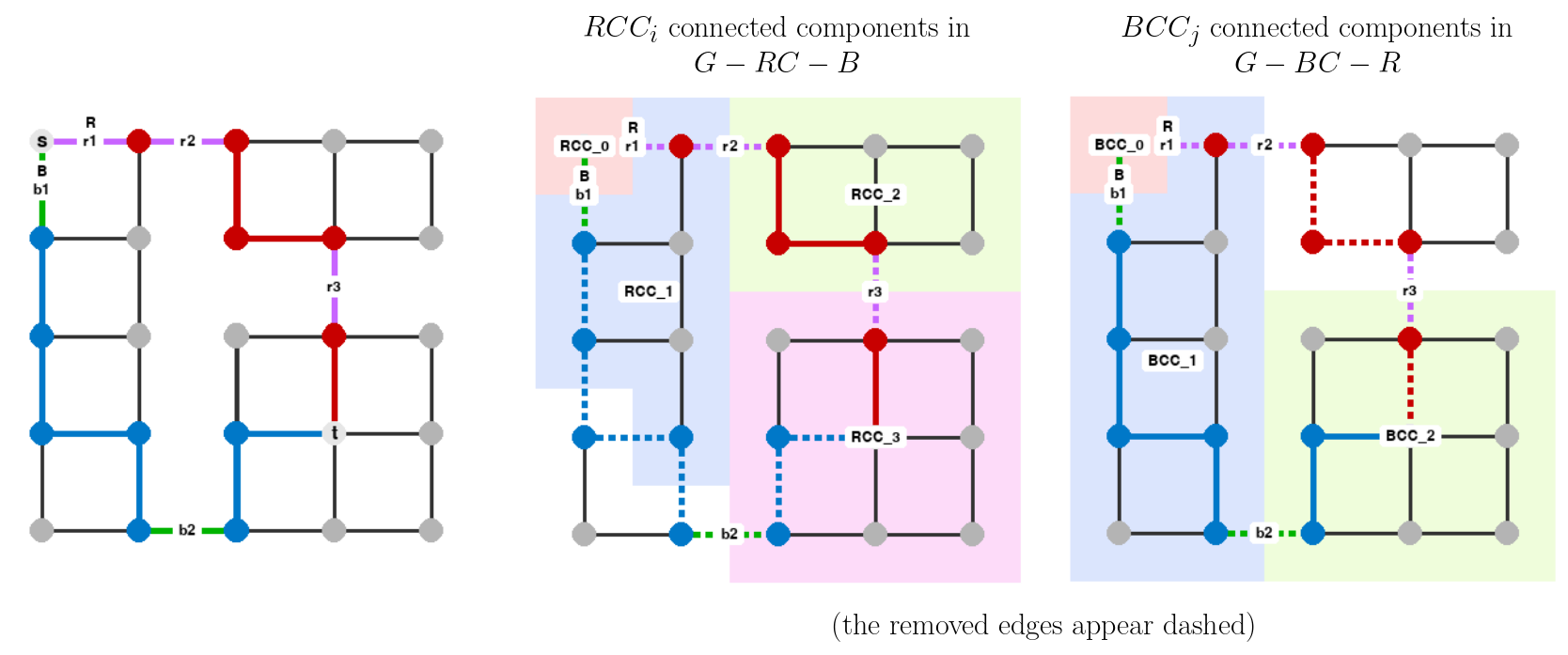
To compute the cross edges in the path-segment graph, we first label all the nodes in the original graph according to which RCC_i and BCC_j connected components they belong to. Then, we add a cross edge between rs_i and bs_j in the path-segment graph if and only if there is a node in the original graph that is in both RCC_i and BCC_j.

Here is another example of path-segment graph:

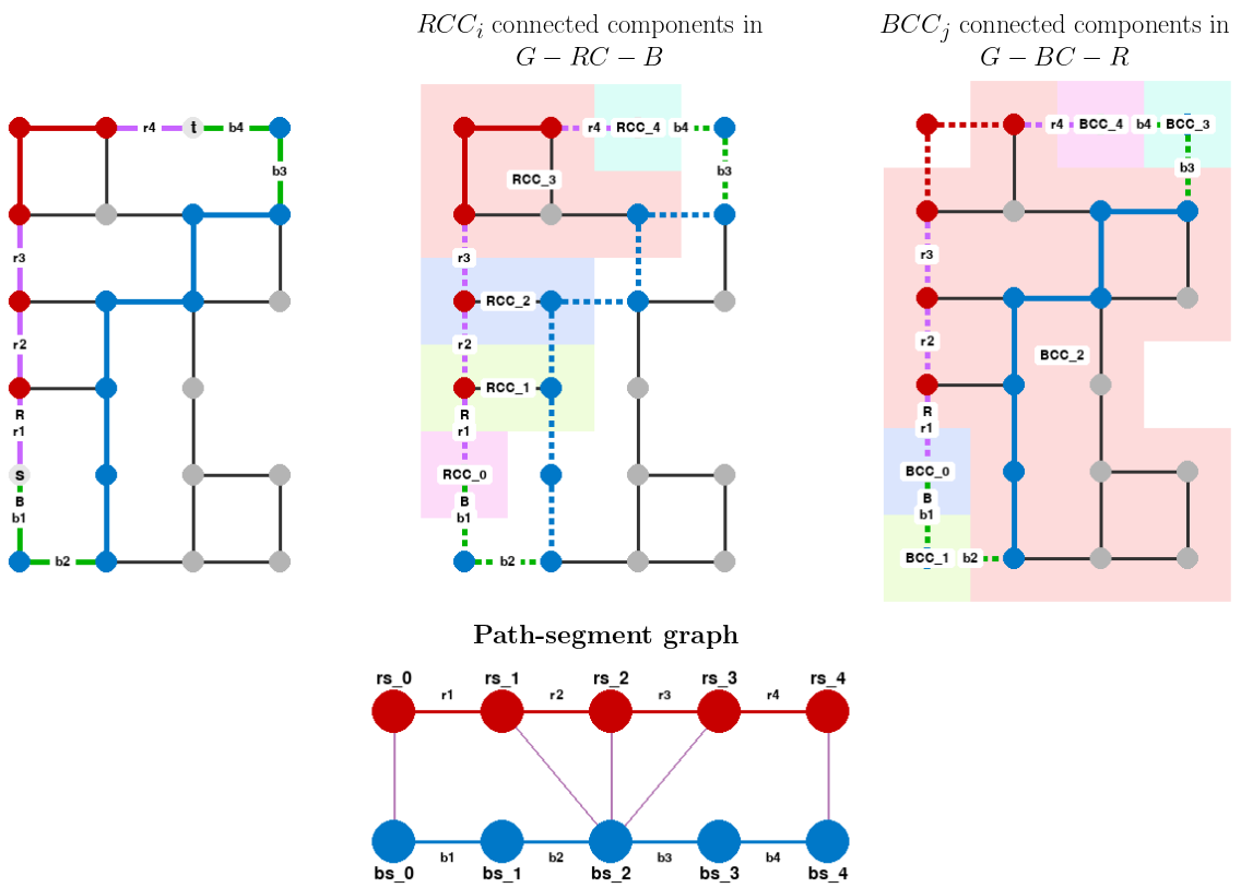
In this graph, the essential pairs are (r1, b1), (r1, b2), (r4, b3), and (r4, b4).

This example shows that there can be candidates that are not part of any essential pair (r2 and r3 in this case).

The path-segment graph can be computed in linear time. In particular, it has at most V cross edges, since each cross edge (rs_i, bs_j) requires a node in the original graph contained in both RCC_i and BCC_j.

Reducing connectivity in the original graph to connectivity in the path-segment graph

Starting from this section, we need one more bit of notation: we use the subindex >=i to indicate "all subindices greater than or equal to i" and the subindex <i to indicate "all subindices less than i".

The following lemma shows that instead of checking if a candidate pair, (ri, bj), disconnects s and t in the original graph, we can check if it disconnects rs_0 and rs_k in the path-segment graph. This makes our job easier since the path-segment graph is structurally simpler than the original graph.

Lemma 1: A candidate pair (ri, bj) is essential if and only if it disconnects rs_0 and rs_k in the path-segment graph.

In other words:

1. If removing (ri, bj) disconnects rs_0 and rs_k in the path-segment graph, then it disconnects s and t in the original graph.
2. If removing (ri, bj) does not disconnect rs_0 and rs_k in the path-segment graph, then it does not disconnect s and t in the original graph.

Proof:

Starting with (2), if there is a path from rs_0 to rs_k in the path-segment graph that does not use ri or bj, we can turn it into an s-t path in the original graph that does not use ri or bj either: we follow one of the paths, say R, until we have to use a cross edge in the path-segment graph, say, (rs_x, bs_y). We know that RCC_x and BCC_y share at least a node, v, so we can find a path from one of the nodes in the path segment for rs_x to v and from v to one of the nodes in the path segment for bs_y. We can then continue following the other path, B, until we reach t or need to use another cross edge, which we can handle in the same way.

For (1), we want to show that there is no s-t path in the original graph without ri and bj.

By definition, without ri, there is no way to get to RCC_>=i without using blue edges. However, using blue edges before bj still does not allow us to reach any nodes in RCC_>=i (otherwise, rs_0 and rs_k would still be connected in the path-segment graph thanks to a cross edge).

(The proof for (1) is admittedly hand-wavy, I may have to revisit it.)

Compressing the path-segment graph

The following lemma will allow us to do a final transformation to the path-segment graph to further simplify its structure (the exact reason will be clear later).

Lemma 2: The following two statements are equivalent: (a) A candidate pair (ri, bj) is essential; (b) for every cross edge (rs_x, bs_y) in the path-segment graph, ri and bj are both on the same side of that cross edge (i <= x and j <= y, or i > x and j > y).

Proof:

• (a) => (b) direction: Assume, for the sake of contradiction, that (ri, bj) is essential but there is a cross edge (rs_x, bs_y) such that i <= x and j > y. Then, we can go from rs_0 to bs_0, from bs_0 to bs_y, from bs_y to rs_x, and from rs_x to rs_k. This contradicts that (ri, bj) is essential. The other case is symmetric.
• (b) => (a) direction: cross edges of the form (s1_<i, s2_<j) do not allow us to "skip" over ri and bj. Cross edges of the form (s1_>=i, s2_>=j) have two endpoints neither of which can be reached from rs_0 in the first place.

Lemma 2 is important for the following reason:

If we have a chain of edges in the path-segment graph, rx, ..., ry, without any cross edges coming out of the nodes between them, then all the edges in the chain have all the same cross edges on each side. A corollary of Lemma 2 is that combining any of these edges with a blue candidate, bj, has exactly the same effect on whether rs_0 and rs_k stay connected. Thus, we can compress the chain into a single edge, r_x,y, as shown in the figure:

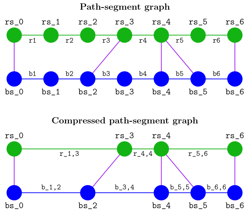
In this path-segment graph, we compressed r1, r2, and r3 into r_1,3, left r4 alone (relabeled as r_4,4), and compressed r5 and r6 into r_5,6. The blue candidates got compressed similarly.

The result is a new graph, which we call the compressed path-segment graph. It is similar to the path-segment graph, but with potentially fewer nodes and edges.

We call a pair of edges in the compressed path-segment graph, (r_x,y, b_z,w), essential if they disconnect r_0 and r_k. What that means is that any red candidate compressed into r_x,y forms an essential pair with any blue candidate compressed into b_z,w.

The compressed path-segment graph has the property that every node is adjacent to at least one cross edge. This is important for one reason:

In the normal path-segment graph, an edge in the top path could form an essential pair with many edges in the bottom path, leading to a potentially quadratic number of essential pairs. In the compressed path-segment graph, each edge in the top path can only form an essential pair with at most one edge in the bottom path. This is because of Lemma 2: there are cross edges between every pair of edges in the bottom path, so only one of them can match the position of the top edge relative to all the cross edges.

Finally, we reached a point where we can store all the essential pairs in O(V) space. We can only do this because each edge of the compressed path-segment graph represents potentially many candidates in the original graph.

Now, we just need to compute them in linear time.

Computing essential pairs in the compressed path-segment graph

We can use a straightforward two-pointer algorithm, with one pointer for each path. The red pointer starts at the edge r_1,x and the blue pointer starts at the edge b_1,y. For each pointer, we keep track of which cross edges we've already passed. Then, we have a case analysis:

• If both pointers have passed the same cross edges, mark the current edge pair as essential, and advance both pointers.
• If the red pointer has passed any cross edges that the blue pointer hasn't passed, advance the blue pointer.
• If the blue pointer has passed any cross edges that the red pointer hasn't passed, advance the red pointer.

With this method, we can find and store all the essential pairs in the compressed path-segment graph in O(V) time.

To know if a pair of candidates (ri, bj) in G is essential, we check if the compressed edges they belong to form an essential pair in the compressed path-segment graph.

Implementation

In this section, we'll see how all the pieces fit together by designing the full data structure as described at the beginning of the post.

The data structure is implemented in TypeScript here. There is also the brute-force solution, tests, the visualization tool (in Python), and a little benchmark we'll use for the next section.

Construction:

The only constraint on G is that s and t are connected and different.

Input: G (adjacency list), s, t

Find a path P from s to t in G
Find the bridges in G
Store the set of bridges that are in P
Find the biconnected components of G
For each biconnected component crossed by P with >2 nodes:
  Find two node-disjoint paths from the entry point of P to the exit point of P
  Compute the red and blue candidates
  Compute the path-segment graph
  Compute the compressed path-segment graph
  Find all the essential pairs in the compressed path-segment graph with 2 pointers
  Store the essential pairs in the compressed path-segment graph
  For each red or blue candidate, store the following information:
    - The biconnected component
    - The color (red or blue)
    - The index of the compressed edge it belongs to

Time and space: O(V + E).

Query:

Input: e1, e2 (edge pair)
Output: true if (e1, e2) is essential, false otherwise

If e1 is a bridge in P or e2 is a bridge in P:
  return true
If e1 is not a candidate or e2 is not a candidate:
  return false
return true if:
  - e1 and e2 are in the same biconnected component, and
  - e1 and e2 have different colors, and
  - their compressed edges form an essential pair
else return false

Time and space: O(1).

Benchmark

I generated 10 random 30x30 grid graphs, where each edge is present with probability 0.5. For each graph, I picked s and t randomly, making sure that s and t were connected.

I then initialized the data structure for each graph and queried it with every edge pair in the graph. I also ran all the queries with the brute-force solution.

Here are the results:

Benchmark Results (30x30 grid, P=0.5, Iterations=10):
──────────────────────────────────────────────────────────────────────────────────────
| Algorithm            | Construction (ms)  | Query (ms)         | Total (ms)         |
──────────────────────────────────────────────────────────────────────────────────────
| Brute force          | 0.015              | 3138.044           | 3138.059           |
| Optimized            | 1.368              | 13.236             | 14.604             |
──────────────────────────────────────────────────────────────────────────────────────

Speedup (Naive/Optimized):
Query:        237.09x
Total:        214.88x

Average query time per edge pair:
Naive:     0.002024 ms
Optimized: 0.000009 ms

Total Queries:             15506574
Positive Queries:          763483 (4.92%)

Average number of edges per graph:      1761
Average number of edge pairs per graph: 1550657

The bigger the graph, the more queries we can do, and thus the more the preprocessing pays off. With 11x11 grid graphs, which is the standard size for the Wall Game, we do only ~15k queries per graph, and the speedup is only about 6x.

For both 30x30 and 11x11 grid graphs, the construction of the data structures is about 3 orders of magnitude slower than solving a single query directly with a graph traversal. This is surprising, given the optimized data structure only does a constant number of graph traversals (about 10). My theory is that the overhead comes from allocating memory (e.g., for the various derived graphs; the keyword new appears ~30 times in the code) and from the use of hash sets and maps.

Optimizing the code was not the main point of this post. It can be optimized further by doing things like:

• Pre-allocating and reusing the visited and stack arrays across all the functions that need to do some kind of graph traversal.
• Not explicitly constructing the directed graph in findTwoNodeDisjointPaths().
• Not explicitly constructing graphs like G - R, G - B, G - R - BC, and G - B - RC. Instead, we can pass around a set of "disallowed" edges. (The path-segment graph and the compressed path-segment graphs are already not constructed explicitly.)
• Avoiding hash sets and maps with edges as keys. Instead, edges could be mapped to contiguous integers from 0 to E - 1 (I already avoided using sets and maps when the keys are integers starting at 0, like node indices).
• Choosing a better language for low-level optimizations...

---

Want to leave a comment? You can post under the linkedin post or the X post.