A Fully Annotated NanoGPT Script

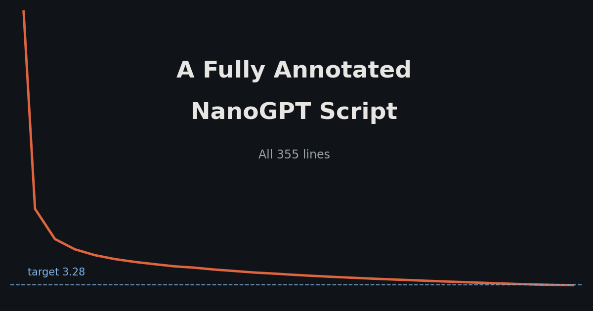
What does it actually take to train a language model?

In 2024, Andrej Karpathy reproduced GPT-2 (2019) with a small script. Training it to GPT-2's quality level took the equivalent of 45 minutes on 8 NVIDIA H100 GPUs. Then, Keller Jordan turned this into a competition, the NanoGPT speedrun: reach the same bar (a score of 3.28 on a held-out test, defined later) as fast as possible on the same hardware. The community has since driven it from 45 minutes down to under 90 seconds.

The script in this post is not the current record, but it is far faster than Karpathy's starting point. Prime Intellect prepared this script as a cleaned-up baseline for an open-ended experiment (can agents running autonomously bring the record down?) It plays the speedrun track scored by number of training steps rather than wall-clock time, which makes results comparable across hardware. Karpathy's version took 19,560 steps; this one took 3,500. The record is now at 2,690 (June 2026).

All 355 lines appear below, untouched and in order.

Glossary

Here's the basic vocab when talking about LLMs; we'll use it throughout.

• Transformer: the neural network architecture built in this post; it's behind GPT-2 and essentially all modern LLMs. It predicts the next token in a sequence.
• Token: LLMs take tokens as input, not text. A program called a tokenizer converts text into tokens, which stand for a word or word fragment. GPT-2 (and this model) have 50,257 tokens: 256 base tokens for single bytes, 50,000 "learned" multi-byte ones, and 1 special end-of-text marker.
• Parameters (also called weights): the numbers inside the model that training adjusts. This model has about 162 million parameters stored as a mix of 16-bit and 32-bit floating-point numbers.
• Training step: one full model update cycle: process one batch, compute the gradient, nudge every parameter once. The script reaches GPT-2's level in 3,500 steps.
• Batch: the data consumed by one training step, 524,288 tokens (fixed by the speedrun rules). Over 3,500 steps, that's 1.8B tokens, with no repeats; the model sees each training token once.¹
• Gradient: for each parameter, the direction and steepness by which changing it would reduce the loss.
• Loss: a measure of how wrong the model's predictions are; lower is better. The standard loss measure used for transformers is called cross-entropy.
• Validation loss: the loss measured on held-out text the model never trained on (the held-out text is fixed by the speedrun). The speedrun target is 3.28.

Overview

The script has 3 sequential phases:

1. Prepare examples. Load 1.8 billion tokens of web text and cut them into batches; the text itself is the answer key, because the model's job is to guess each next token.
2. Build the model. Initialize a transformer with 162 million parameters. Given a batch, it produces, at every position, a score for each of the 50,257 possible next tokens.
3. Train. Run 3,500 training steps, coordinating the work across up to 8 GPUs. Every 125 steps, pause and measure the validation loss.

Part 0: The header

"""
train_gpt_simple.py

This file descends from the [NanoGPT speedrun](https://github.com/KellerJordan/modded-nanogpt).
It was prepared as a simplified version of the speedrun for use in neural net optimization research.
"""

import os
import sys
with open(sys.argv[0]) as f:
    code = f.read() # read the code of this file ASAP, for logging
import uuid
import time
from pathlib import Path

import torch
from torch import Tensor, nn
from torch.optim import AdamW
import torch.nn.functional as F
import torch.distributed as dist

Notes:

• The odd-looking with open(sys.argv[0]) line reads the script's own source code into a string. Near the end of the setup section, the script writes this string into its log file. That way, every training run permanently records exactly which code produced it. It's a habit worth stealing.
• PyTorch (torch) is the dominant library for building neural networks. It gives you arrays that live on the GPU with fast math operations, and autograd: it records every computation you run and can then walk the recording backwards to compute gradients for you.
• nn: the neural-network building-blocks submodule.
• torch.nn.functional (imported as F): the same operations as nn but as pure functions; used when there is no learnable state involved.
• Tensor is the class of PyTorch's arrays. Used only for type hints.
• torch.distributed (imported as dist) coordinates several GPUs working on the same training run.
• AdamW is an off-the-shelf optimizer (Part 3).

Part 1: The data loader

The model learns from FineWeb, a public dataset of text scraped from the web and cleaned up. The text has already been converted to tokens before this script ever runs; the token files sit on disk in a simple binary format.

Recall that a token is a number standing for a word or word fragment. For example, "The cat" becomes [464, 3797] ("The" and " cat").

########################################
#              Dataloader              #
########################################

def _load_data_shard(file: Path):
    header = torch.from_file(str(file), False, 256, dtype=torch.int32) # header is 256 int32
    assert header[0] == 20240520, "magic number mismatch in the data .bin file"
    assert header[1] == 1, "unsupported version"
    num_tokens = int(header[2]) # number of tokens (claimed)
    with file.open("rb", buffering=0) as f:
        tokens = torch.empty(num_tokens, dtype=torch.uint16, pin_memory=True)
        f.seek(256 * 4)
        nbytes = f.readinto(tokens.numpy()) # avoid bytes->array copy
        assert nbytes == 2 * num_tokens, "number of tokens read does not match header"
    return tokens

This function reads one shard, a file holding 100 million tokens (about 200 MB). After 256 numbers of header, the tokens follow as uint16 (unsigned 16-bit integers) values; they can hold values up to 65,535, plenty for 50,257 token IDs.

The header starts with the "magic number" 20240520 (a date). Checking it catches the embarrassing failure mode of pointing the script at the wrong kind of file. The remaining lines read the token payload straight into a preallocated buffer. pin_memory=True asks for a special kind of main memory that the GPU can pull from at full speed (we dug into pinned memory in the Wall Game inference deep dive post), and f.readinto fills it without any intermediate copies.²

def distributed_data_generator(filename_pattern: str, batch_size: int, seq_len=1024):
    world_size = dist.get_world_size()
    rank = dist.get_rank()
    files = sorted(Path.cwd().glob(filename_pattern))
    assert batch_size % world_size == 0
    local_batch_size = batch_size // world_size
    file_iter = iter(files)
    tokens, pos = _load_data_shard(next(file_iter)), 0
    while True:
        if pos + batch_size + 1 >= len(tokens):
            tokens, pos = _load_data_shard(next(file_iter)), 0
        buf = tokens[pos + rank * local_batch_size:][:local_batch_size + 1]
        inputs = buf[:-1].to(device="cuda", dtype=torch.int32, non_blocking=True)
        targets = buf[1:].to(device="cuda", dtype=torch.int64, non_blocking=True)
        pos += batch_size
        yield inputs.view(-1, seq_len), targets.view(-1, seq_len)

This generator hands out training batches forever (yield inside while True).

It is also our first time seeing multi-GPU coordination. The script may run on 1, 2, 4, or 8 processes. Each process runs its own copy of this script. The copies are given a rank (rank 0, rank 1, ...) and the total count is the world size. Each process is assigned its own GPU and holds an identical model, but must learn from different text (otherwise the extra GPUs would add nothing).

That is what the slicing does. Each step consumes batch_size tokens globally (524,288). Then, each rank takes its own local_batch_size slice of that, offset by its rank.

The + 1 in the buffer slicing is the heart of LLM training. The buffer is one token longer than the rank's share of the batch so that inputs and targets have the right length:

• inputs = the buffer without its last token,
• targets = the buffer without its first token.

So targets is inputs shifted left by one: at every position, the target is the token that came next in the real text. targets[i] is the token to predict after inputs[0] ... inputs[i]. The two arrays provide one training data point for each token in the batch. There's no separate source of labels - the text itself is the answer key.

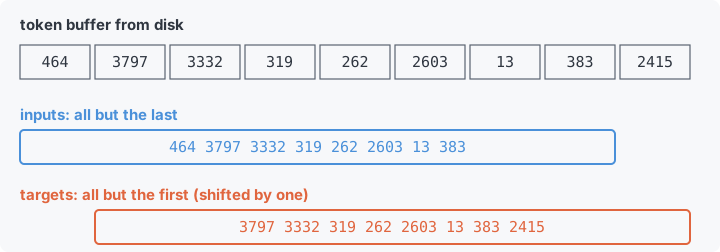
The conditional if pos + batch_size + 1 >= len(tokens) makes it so that when the current shard runs low, we move to the next one, discarding the last few tokens.

The final view(-1, seq_len) reshapes the flat token stream into rows of 1,024 tokens each. The model will treat each row as an independent piece of text and never look across rows. A row is usually called a sequence, and 1,024 is the sequence length.

The batch dimension is the number of sequences per GPU:

batch dimension = batch size / (world size * sequence length)

For example, with 8 GPUs, the batch dimension is 524288 / (8 * 1024) = 64.

From here on, data moving through the model has a shape like B × T: B sequences (the batch dimension) of T = 1,024 tokens each.

Two dtype details: inputs become int32 and targets int64, simply because those are the integer types the two consuming operations (the embedding lookup and the loss function) require. The non_blocking=True copies let the GPU fetch the next batch while still computing on the current one.

Part 2: The model

The model has this shape:

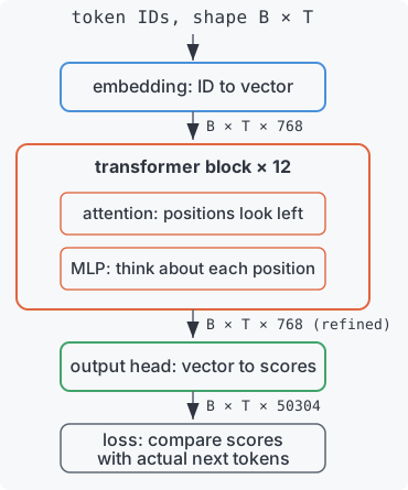
Each token ID becomes a list of 768 numbers - we say it's embedded as a vector in a 768-dimensional space. Twelve transformer blocks (identical structure, different parameters) refine those embeddings, letting information flow from earlier positions to later ones. At the end, the embedding at each position is converted into 50,304 scores, one per possible next token, and the scores are graded against what actually came next.

The vectors' length (768) is the model dimension. A grid of vectors, like our B × T × 768 batch, is a tensor, PyTorch's basic object: an array with any number of dimensions that lives on the GPU. The model's 162 million parameters live in grids like these too, and learning happens by nudging them so the scores get less wrong.

The model predicts next tokens within each sequence. The B dimension is just parallel, independent computations.

Normalization

########################################
#             Architecture             #
########################################

def norm(x: Tensor):
    return F.rms_norm(x, (x.size(-1),))

class RMSNorm(nn.Module):
    def __init__(self, dim):
        super().__init__()
        self.gains = nn.Parameter(torch.ones(dim))

    def forward(self, x):
        return (norm(x.float()) * self.gains).type_as(x)

These two snippets are two flavors of normalization. Deep networks are towers of multiplications; without periodic rescaling, numbers drift toward huge or tiny as they pass through the layers, and learning becomes unstable.

Without getting into the math, rms_norm (root mean square normalization) shrinks or stretches the vector so its entries hover around [-1, +1], without changing its direction.

The plain function norm is the bare rescaling. The (x.size(-1),) argument says to normalize along the last axis of the tensor: each token's 768-entry vector is rescaled independently, so tokens do not influence each other's rescaling.

The class RMSNorm additionally multiplies by gains, a learnable per-channel scale (initialized to all ones). A channel is one position in the 768-entry vector: the same slot across all tokens, like "entry 137 of every vector". The gains let the model learn to amplify or mute individual channels after the rescaling.

RMSNorm is our first PyTorch module: in PyTorch, a module is a component that owns parameters (here gains) and defines a forward computation. nn.Parameter marks a tensor as "adjust me during training".

One recurring pattern makes its first appearance in RMSNorm.forward: cast-up, compute, cast-down. To understand it, first we need to define the bfloat16 type.

A bfloat16 number is a 16-bit floating-point number designed by Google Brain (the "b" stands for "brain"). Compared to the standard 32-bit float32, it halves the size, doubling how fast numbers move around the GPU. However, it keeps float32's full range of magnitudes (tiny to astronomically large) and gives up precision instead, keeping only 2 to 3 significant decimal digits. This means that when casting down from float32 to bfloat16, the value never overflows/underflows, but loses some precision. This is the right trade for neural networks because they tolerate imprecise values well.

The model stores and moves most numbers as bfloat16's. In RMSNorm.forward, x.float() casts up to float32, and the following .type_as(x) casts back down to bfloat16. The idea is to do delicate arithmetic (like averaging squares) in precise float32, then convert back to fast bfloat16 for transport. You will see this dance in several places.

Linear layers

class Linear(nn.Linear):
    def __init__(self, in_features, out_features):
        super().__init__(in_features, out_features, bias=True)

    def forward(self, x):
        return F.linear(x, self.weight.type_as(x), self.bias.type_as(x))

A linear layer is the workhorse of all neural networks: it multiplies its input vector by a matrix of learned weights (and adds a learned offset, the bias). This is also how vectors change size: a Linear(in_features, out_features) transformation turns a vector of length in_features into one of length out_features.

Most "knowledge" in a transformer lives in these matrices.

This subclass exists only to apply the casting policy: weights are stored in float32, but type_as(x) converts them to bfloat16 on the fly to match x. Here, x is a tensor flowing through the network, as opposed to the parameters stored in it; these tensors are called activations. In this model, activations travel as bfloat16's.

Rotary position encoding

Attention, coming up shortly, processes all past tokens at the same time; this is the crucial piece that makes transformers really efficient compared to previous architectures, which would process the input in order from left to right. But attention's math treats the past tokens as an unordered bag: nothing in it distinguishes "the token right before me" from "the token 500 positions ago".

So, how does the model know that token 5 comes right after token 4? The answer is position encoding: a way of stamping "where am I in the sequence" onto the token's embedding itself.

class Rotary(nn.Module):
    def __init__(self, dim: int):
        super().__init__()
        # half-truncate RoPE (w/ base freq tuning)
        angular_freq = (1 / 1024) ** torch.linspace(0, 1, steps=dim//4, dtype=torch.float32)
        self.register_buffer("angular_freq", torch.cat([angular_freq, angular_freq.new_zeros(dim//4)]))

    def forward(self, x_BTHD: Tensor):
        pos = torch.arange(x_BTHD.size(1), dtype=torch.float32, device=x_BTHD.device)
        theta = torch.outer(pos, self.angular_freq)[None, :, None, :]
        cos, sin = theta.cos(), theta.sin()
        x1, x2 = x_BTHD.to(dtype=torch.float32).chunk(2, dim=-1)
        y1 = x1 * cos + x2 * sin
        y2 = x1 * (-sin) + x2 * cos
        return torch.cat((y1, y2), 3).type_as(x_BTHD)

This is RoPE (rotary position encoding), the modern standard, and the densest few lines in the file.

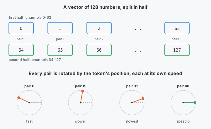
The idea is to pair up the channels in a vector so they can be seen as 2D points. Here we are dealing with vectors of size 128 (we'll see why later); the channel pairs are (0, 64), (1, 65), and so on. Then, we rotate each point by an angle proportional to the token's position in the sequence: the point for the token at position 10 is spun twice as far as the point for the token at position 5.

The payoff comes from the fact that attention scores one token against another with a dot product (Attention section); rotating a point never changes its length, so the only thing these rotations can change in that dot product is the angle between the two points. Rotate each token's point by its position, and the angle between two tokens shifts in proportion to the gap between their positions. So, the score a token gives an earlier one depends on how many steps back it sits, not on either token's absolute location - usually what matters in language ("the word just before me", not "the word at position 412"). Relative position is baked into every comparison for free, with nothing learned. (That is why register_buffer is used: it stores a tensor on the module, saved alongside it, that is not a trainable parameter.)

We rotate multiple points (channel pairs) per token; different points rotate at different speeds, from fast (1 radian per position) down to slow (1/1024 radians per position). That is the angular_freq line: a geometric ramp of rotation speeds. Fast channels distinguish "1 token apart" from "2 tokens apart"; slow channels distinguish "100 apart" from "500 apart".

Standard RoPE spins every pair. This "half-truncate" variant spins only the first half and leaves the rest alone; they carry no position information and are free to encode pure content. This happened to improve training.

Notes:

• The new_zeros concatenation sets the second half of the rotation speeds to zero; that's the "half-truncate" tweak.
• The odd variable name x_BTHD is a naming convention: each letter names one axis of the 4-axis input tensor: Batch (sequence index inside the batch), Time (position in the sequence), Head, and Dimension. The rotation only reads T (the position, which gets converted to angles) and acts on D (the entries being rotated). H and D are explained in the next section, where this class is used.
• forward computes the rotation angle for every position and applies the standard 2D rotation formula to each pair. The rotation is computed in float32 and cast back down: the same cast-up, compute, cast-down pattern as in RMSNorm.

Attention

Attention is the only place where positions in the input sequence 'exchange' information.

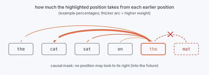
In an attention block, we compute three vectors for each of the 1024 positions, by multiplying each position's current vector by three learned matrices. The vectors are:

• a query: "here is what I am looking for",
• a key: "here is what I contain",
• a value: "here is what I will hand over if you pick me".

Each position takes its query and compares it against the keys of all earlier positions (using dot product, a similarity measure for vectors based on how aligned they are). The comparison scores are turned into percentages, and the position receives the percentage-weighted average of those positions' values. Strong query-key matches contribute a lot; weak ones barely at all.

Example: when the model processes "the cat sat on the ___", the query at the blank can align with the key at "cat", pulling in the value which nudges the vector in a direction that increases the probability of guessing a cat-appropriate word.

class CausalSelfAttention(nn.Module):
    def __init__(self, dim: int, head_dim=128):
        super().__init__()
        self.num_heads = dim // head_dim
        self.head_dim = head_dim
        hdim = self.num_heads * self.head_dim
        self.q = Linear(dim, hdim)
        self.k = Linear(dim, hdim)
        self.v = Linear(dim, hdim)
        self.proj = Linear(hdim, dim)
        self.rotary = Rotary(head_dim)

    def forward(self, x: Tensor):
        B, T = x.size(0), x.size(1)
        q = self.q(x).view(B, T, self.num_heads, self.head_dim)
        k = self.k(x).view(B, T, self.num_heads, self.head_dim)
        v = self.v(x).view(B, T, self.num_heads, self.head_dim)
        q, k = norm(q), norm(k)
        q, k = self.rotary(q), self.rotary(k)
        y = F.scaled_dot_product_attention(q.transpose(1, 2), k.transpose(1, 2),
                                           v.transpose(1, 2), scale=0.12, is_causal=True).transpose(1, 2)
        y = y.contiguous().view(B, T, self.num_heads * self.head_dim)
        y = self.proj(y)
        return y

Reading it top to bottom:

• The model dimension 768 is split into 6 heads of 128 channels each. Each head runs the whole query/key/value mechanism independently, with its own learned matrices. Six heads means six different "conversations" per position at once: one head might track grammar, another might track which entities were mentioned. (H and D in the earlier _BTHD are the head index and the channel within it.)
• q, k, v are the three linear layers producing queries, keys, and values; the view in forward reshapes them from B x T x 768 to B x T x 6 x 128.
• norm(q), norm(k): queries and keys are RMS-normalized before comparison. This "QK norm" is a stability trick: it caps how extreme the comparison scores can get, which keeps the percentages well-behaved.
• self.rotary applies the position-stamping rotation from the previous section to queries and keys. Values are left alone: position influences who gets picked, not what they hand over.
• F.scaled_dot_product_attention is PyTorch's built-in that executes the recipe from the top of this section (compare queries to keys, turn scores into percentages, add values weighted by percentages) in one highly optimized GPU kernel (a kernel is a single program launched on the GPU; fusing the whole compare-weigh-average procedure into one avoids writing the large intermediate results out to GPU memory between steps). is_causal=True enforces the "earlier positions only" rule, called causal masking: position 7 may look at 0 through 7, never at 8 or later. This is so that the model cannot peek at the answer.
• scale=0.12 multiplies the comparison scores before they become percentages. The textbook value would be 1/sqrt(128), about 0.088; 0.12 is what worked out the best while tuning for the speedrun.
• The transpose calls put the axes in the order the built-in expects (heads before positions), and .contiguous() reorganizes memory after transposing so the final reshape is legal.
• Finally, the six heads' outputs are glued back into one 768-vector and passed through a last linear layer, proj (projection), which mixes what the heads gathered. (Remember this proj; something curious happens to it at initialization time, in Part 5.)

The MLP

class MLP(nn.Module):
    def __init__(self, dim: int):
        super().__init__()
        hdim = 4 * dim
        self.fc = Linear(dim, hdim)
        self.proj = Linear(hdim, dim)

    def forward(self, x: Tensor):
        x = self.fc(x)
        x = x.relu().square()
        x = self.proj(x)
        return x

If attention transfers information between positions, the MLP (multi-layer perceptron) processes each position by itself:

• self.fc(x) ("fully connected", from an old naming convention) expands each 768-vector to 3,072 channels (four times wider) with a linear transformation.
• x.relu().square() applies a nonlinear operation: ReLU (rectified linear unit) zeroes out negatives, and then we square what remains. Without this nonlinear step, the whole MLP would collapse into one big linear transformation. I wrote about why non-linearity is key. The use of squared-ReLU over more common options like plain ReLU or GELU (the variant used in GPT-2) is a speedrun empirical win.
• self.proj(x) (projection) compresses back to 768.

The MLP matrices have twice as many parameters as the attention matrices. Interpretability research suggests this is where much of the "world knowledge" is stored, something I wrote about here.

The block

class Block(nn.Module):
    def __init__(self, dim: int):
        super().__init__()
        self.attn = CausalSelfAttention(dim)
        self.mlp = MLP(dim)
        self.norm1 = RMSNorm(dim)
        self.norm2 = RMSNorm(dim)

    def forward(self, x: Tensor):
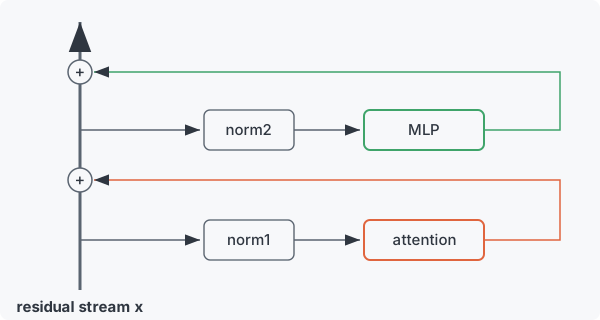
        x = x + self.attn(self.norm1(x))
        x = x + self.mlp(self.norm2(x))
        return x

A block wires one attention and one MLP together.

Note that forward adds attn(...) and mlp(...) to the current vectors flowing through the network, instead of replacing them. This is called the residual stream. Each step takes a copy of the vectors, computes something, and nudges the vectors with the result. Learning a useful "correction" is easier than "reconstructing" everything the previous layers did.

The residual stream helps training. During backpropagation, the error signal (or "gradient") travels backward and gets multiplied by each layer's local derivative; if every layer is allowed to shrink it multiplicatively, almost nothing reaches the earlier layers. But the derivative of x + f(x) with respect to x is 1 + f'(x). So, the 1 passes the gradient through unchanged. This means that every layer receives a full-strength copy of the error signal, plus an additive (not multiplicative) term.

norm1 and norm2 normalize the copies going into a sublayer; this practice is universally used for stability.

The full model

class GPT(nn.Module):
    def __init__(self, vocab_size: int, num_layers: int, model_dim: int):
        super().__init__()
        self.embed = nn.Embedding(vocab_size, model_dim).bfloat16()
        self.blocks = nn.ModuleList([Block(model_dim) for _ in range(num_layers)])
        self.proj = Linear(model_dim, vocab_size)
        self.norm1 = RMSNorm(model_dim)
        self.norm2 = RMSNorm(model_dim)

    def forward(self, inputs: Tensor, targets: Tensor):
        x = self.norm1(self.embed(inputs))
        for block in self.blocks:
            x = block(x)
        logits = self.proj(self.norm2(x)).float()
        logits = 15 * logits * (logits.square() + 15**2).rsqrt()
        return F.cross_entropy(logits.view(targets.numel(), -1), targets.view(-1), reduction="sum")

In __init__, we declare all the parts with parameters:

• The embedding is the token-ID-to-vector table: 50,304 rows (one per possible token), 768 columns (the model dimension). Recall that the tokenizer's actual vocab size is 50,257, but here it's bumped to the next value divisible by 128; GPUs run matrix operations measurably faster when the sizes divide evenly into their hardware tile sizes. The 47 extra rows are ignored.
• The 12 blocks.
• proj, the output head: the final linear layer mapping each position's 768-vector to 50,304 numbers, one per token in the vocabulary. These raw scores are called logits. Bigger logit = the model considers that token a more likely next token.³
• Two normalization layers.

In forward, recall that both inputs and targets are B x T, where B is the sequences per GPU and T = 1,024 is the sequence length.

We do the full forward journey for each sequence: embed, normalize, the twelve blocks, normalize again, and project to logits in float32.

The 15 * logits * rsqrt(...) line is logit soft-capping: a smooth squash that keeps every logit in the range -15 to +15 (for small values it changes almost nothing; extreme values get compressed toward the cap). Uncapped logits let the model chase overconfidence with huge scores, which destabilizes the loss; the cap takes that failure mode away.

The last line grades the predictions using cross-entropy, the standard scoring rule for probabilistic predictions. Cross-entropy first converts the logits into probabilities via softmax, which is like a soft version of max(); higher scores get exponentially higher probabilities, so any score that's not close to the maximum gets a really small probability. Then, it looks up what probability the model assigned to the actual next token, and takes the negative logarithm of that probability.

• If the target has a probability of 1, the loss is 0.
• If the probability is 10%, the loss is 2.3.
• If the probability is 3.8%, the loss is 3.28.

The speedrun's goal is 3.28 average cross-entropy per token on held-out text. It is roughly equivalent to the model assigning the true next token 3.8% probability (in geometric-average terms), which sounds bad until you remember there are over 50k candidates and many tokens are genuinely unpredictable.

Note reduction="sum": it returns the total loss over all tokens, not the average. Using sums keeps the multi-GPU math clean, as we can add across GPUs to get the total.

Part 3: The optimizer

The model is now complete; everything from here is how the 162M numbers get updated efficiently.

The naive update rule ("move each parameter by a fixed multiple of its gradient", called gradient descent) works but is slow. This script's biggest departure from the textbook is here: it uses Muon, an optimizer invented by Keller Jordan for this speedrun in 2024.

########################################
#              Optimizer               #
########################################

def zeropower_via_newtonschulz5(G: Tensor) -> Tensor:
    assert G.ndim >= 2
    X = G.bfloat16()
    if G.size(-2) > G.size(-1):
        X = X.mT

    # Ensure spectral norm is at most 1
    X = X / (X.norm(dim=(-2, -1), keepdim=True) + 1e-7)
    # Perform the NS iterations, not optimizing for wallclock speed
    a, b, c = 2, -1.5, 0.5
    for _ in range(12):
        A = X @ X.mT
        B = b * A + c * A @ A
        X = a * X + B @ X

    if G.size(-2) > G.size(-1):
        X = X.mT
    return X

This is the mathematical core (you can skip it and still follow the training loop).

It's based on one concept from linear algebra known as SVD (Singular Value Decomposition): a matrix transforms vectors, and every matrix has a set of special direction pairs, one in the input space and one in the output space, such that each of those input directions maps to the corresponding output direction and only gets stretched, not rotated. Each pair is stretched by its own factor, and those factors are known as the matrix's singular values.

The function above takes a matrix and reshapes it so all stretch factors become approximately equal to 1, while keeping the directions untouched. This is called orthogonalization.

Muon does this to gradient matrices (the gradient of one parameter matrix, arranged in the same matrix's shape). The reason is that a raw gradient matrix is typically dominated by a few strong directions, so the interesting-but-faint directions are drowned out. If you take a step along the raw gradient, you mostly re-walk the loud directions over and over. Equalizing the strengths lets every useful direction make progress at once. That is Muon's bet, and empirically it pays off: it reduced the number of steps by roughly a factor of 3.

The implementation is an old numerical trick, Newton-Schulz iteration: instead of computing the orthogonalization exactly, which is slow, we repeatedly apply a fixed polynomial recipe (the a, b, c lines: each round computes a small matrix polynomial of X) that provably pushes all stretch strengths toward 1. We do twelve rounds of matrix multiplication (suitable for GPUs), in compact bfloat16's. Part of the Muon discovery was that this iteration tolerates low precision just fine. The transpose dance at the entry and exit just ensures the matrix is wider than tall during the iteration, the cheaper orientation.

@torch.compile
def muon_update(grad, momentum, mu=0.95, nesterov=True):
    momentum.lerp_(grad, 1 - mu)
    update = grad.lerp_(momentum, mu) if nesterov else momentum
    update = zeropower_via_newtonschulz5(update)
    update *= max(1, grad.size(-2) / grad.size(-1))**0.5
    return update

This is how we compute a full update for one parameter matrix and training step (i.e., based on the loss for one batch). momentum is a matrix of the same size with a running average of each gradient for recent batches: lerp_(grad, 1 - mu) (linear interpolation) blends 5% of the new gradient into 95% of the running average each step. So, the current batch doesn't fully dictate the direction to move the weights; it only influences the direction a tiny bit.

The nesterov line builds the actual update as 5% raw gradient and 95% the just-updated momentum (this is a well known optimization in ML). The blended update is orthogonalized and then scaled by a factor accounting for the matrix's aspect ratio.

The @torch.compile decorator asks PyTorch to fuse this whole recipe into optimized GPU code rather than running it operation by operation from Python.

class Muon(torch.optim.Optimizer):
    def __init__(self, params, lr=0.02, weight_decay=0, mu=0.95):
        assert isinstance(params, list) and len(params) >= 1 and isinstance(params[0], torch.nn.Parameter)
        params = sorted(params, key=lambda x: x.size(), reverse=True)
        defaults = dict(lr=lr, weight_decay=weight_decay, mu=mu)
        super().__init__(params, defaults)

    @torch.no_grad()
    def step(self):
        world_size = dist.get_world_size()
        rank = dist.get_rank()
        for group in self.param_groups:
            params = group["params"]
            params_pad = params + [torch.empty_like(params[-1])] * (world_size - len(params) % world_size)
            for base_i in range(0, len(params), world_size):
                if base_i + rank < len(params):
                    p = params[base_i + rank]
                    state = self.state[p]
                    if len(state) == 0:
                        state["momentum"] = torch.zeros_like(p)
                    update = muon_update(p.grad, state["momentum"], mu=group["mu"])
                    p.mul_(1 - group["lr"] * group["weight_decay"])
                    p.add_(update, alpha=-group["lr"])
                dist.all_gather(params_pad[base_i:base_i + world_size], params_pad[base_i + rank])

The Muon class packages the update into PyTorch's standard optimizer interface (torch.optim.Optimizer). It expects:

1. The parameters to manage, params. PyTorch optimizers like Muon keep a permanent reference to the parameters they are responsible for updating.
2. A step() function, which applies one update step to all the managed parameters.

We use Muon for the 72 2D matrices in the blocks (6 for each of the 12 blocks: attn.q, attn.k, attn.v, attn.proj, mlp.fc, and mlp.proj). Muon only works for 2D matrices because directions and stretch strengths only apply there. For the remaining parameters (the embedding table, the output head, and the various 1D layers) we'll use a different optimizer later.

It introduces a few terms:

• params: the list of 2D parameter matrices from the blocks. __init__ sorts them largest-first, which helps balance the work-sharing below.
• defaults: a dict of hyperparameters lr (learning rate), weight_decay, mu. PyTorch stores them for you.
• param_groups: PyTorch lets you split the parameters into groups that each carry their own hyperparameters, but this class makes only one group.
• state: per-parameter scratch memory the optimizer keeps between steps. Here it holds each matrix's momentum, created lazily on the first step (if len(state) == 0).
• @torch.no_grad(): the update itself is not part of the model's computation, so gradient recording is switched off inside step().

The weight decay (p.mul_(1 - lr * weight_decay)) shrinks every parameter slightly toward zero each step before adding the update. Weight decay is a gentle pressure against parameters growing large, a standard guard against overfitting to quirks of the training data.

Orthogonalizing all those matrices every step is computationally expensive, so ranks split it with a round-robin assignment: assuming we use 8 GPUs, of the model's 72 Muon-managed matrices, rank 0 updates matrices 0, 8, 16..., rank 1 updates 1, 9, 17..., and so on. The sort by size in __init__ helps balance the load. The params_pad line pads the list with dummies so it divides evenly.

Finally, all_gather swaps results between the GPUs so every rank ends up with every updated matrix; they all need the fully updated model for the next learning step. However, each rank only keeps the momentum buffers for the matrices it owns.

Part 4: Setup

This is the part where the script boots the actual run.

########################################
#                Setup                 #
########################################

# torchrun sets these env variables
device = torch.device("cuda", int(os.environ["LOCAL_RANK"]))
torch.cuda.set_device(device)
dist.init_process_group(backend="nccl", device_id=device)
dist.barrier()
# this code can be run equivalently with 1, 2, 4, or 8 gpus.
assert 8 % dist.get_world_size() == 0

This is where the multiple program copies find each other. The launcher (torchrun, see the appendix) starts one copy per GPU and passes each an environment variable saying which local GPU it owns. init_process_group connects the copies through NCCL, the GPU-to-GPU communication library that will carry the all_reduce, all_gather, and broadcast calls. A barrier is a wait-for-everyone point: no rank proceeds until all are ready.

# logging setup
if dist.get_rank() == 0:
    os.makedirs("logs", exist_ok=True)
    logfile = f"logs/{uuid.uuid4()}.txt"
    print(logfile)
def print0(s, console=False, log=True):
    if dist.get_rank() == 0:
        if console:
            print(s)
        if log:
            with open(logfile, "a") as f:
                print(s, file=f)

# we begin by logging this file itself
print0(code)
print0("="*100)
print0(f"Running PyTorch {torch.version.__version__} compiled for CUDA {torch.version.cuda}")
print0(f"Running on device_name={torch.cuda.get_device_name(device)} with world_size={dist.get_world_size()}")
print0("="*100)

print0 is the helper everyone calls; only rank 0 writes logs, the rest do nothing (otherwise, we'd get 8 copies of every line). The first thing we log is the complete source code of the script itself (which we captured in the header) followed by the PyTorch version and hardware. The log file serves as a self-contained record of the experiment.

val_tokens = 20 * 524288
batch_size = 8 * 64 * 1024
mbs = 64
train_loader = distributed_data_generator("data/fineweb10B/fineweb_train_*.bin", batch_size)
val_inputs, val_targets = next(distributed_data_generator("data/fineweb10B/fineweb_val_*.bin", val_tokens))

model = GPT(vocab_size=50304, num_layers=12, model_dim=768).cuda()
model.compile(dynamic=False)

The concrete numbers, finally:

• Each validation pass measures on 20 × 524,288 tokens, about 10.5 million.
• Each training step consumes batch_size = 8 × 64 × 1,024 = 524,288 tokens: with 8 GPUs, that is 64 sequences of 1,024 tokens per GPU per step.
• mbs, the microbatch size of 64 sequences, becomes important in the training loop later.

The batch size and batch contents are fixed by the speedrun rules for the step-count track; thus, the only way to win is to learn more per token. Over 3,500 learning steps, the model reads about 1.8 billion tokens - about five novels' worth of text per step and a small library overall.

The validation data is fetched just once here, with a single next(...): those same ~10.5 million tokens are the held-out set reused for every measurement throughout training.

GPT(vocab_size=50304, num_layers=12, model_dim=768) instantiates the architecture of Part 2.

model.compile asks PyTorch to trace the whole forward-and-backward computation once and generate fused GPU code for it. dynamic=False says that shapes never change, so PyTorch can specialize aggressively. Compilation costs a couple of minutes at startup and pays it back within the first few hundred steps.

Part 5: Initialization and hyperparameters

########################################
#       Init & Optim Hyperparams       #
########################################

# we want to minimize this while still reaching 3.28 val loss
train_steps = 3500

# initialize model parameters
for name, p in model.named_parameters():
    if "proj" in name:
        p.data.zero_()

We initialize every proj layer to zero (each attention's output projection, each MLP's output projection, and the output head). Every other parameter keeps PyTorch's random defaults. This has two effects:

• The residual stream starts as a pass-through. The attention and MLP projections are the last step of each sublayer, so zeroing them means every block adds exactly zero to the stream at step 0. The block stack starts as an identity: input tokens flow through untouched. The blocks then "fade in" from nothing as training moves their projections away from zero.
• The logits start at zero, so the model starts maximally uncertain. With the output head zeroed, every token gets the same score, which softmax turns into equal probability for all 50,257 tokens. A random start, by contrast, would make wild but confident guesses. (It is also why the very first validation loss is about 10.82, the natural log of 50,257: we will see that number in the appendix.)

# create the optimizer(s)
optimizer1 = AdamW([dict(params=[model.embed.weight], lr=0.3),
                    dict(params=[model.proj.weight], lr=1/320),
                    dict(params=[p for p in model.parameters() if p.ndim < 2], lr=0.01)],
                   betas=(0.8, 0.95), eps=1e-10, weight_decay=0, fused=True)
optimizer2 = Muon([p for p in model.blocks.parameters() if p.ndim >= 2],
                  lr=0.025, weight_decay=0.0125)
optimizers = [optimizer1, optimizer2]
assert set(p for opt in optimizers for group in opt.param_groups
           for p in group["params"]) == set(model.parameters())
for opt in optimizers:
    for group in opt.param_groups:
        group["initial_lr"] = group["lr"]

The parameters are split between two optimizers:

• Muon handles the 2D matrices inside the blocks (see Part 3).
• AdamW (an off-the-shelf optimizer imported from PyTorch) handles three groups of parameters: the embedding table, the output head, and everything 1-dimensional (the RMSNorm gains and the biases).

AdamW is the industry-default optimizer; it keeps two running averages per parameter: one of the gradient and one of the squared gradient (its typical magnitude). It steps along the first scaled down by the second, so noisy parameters move more cautiously. The betas (0.8 and 0.95) are the smoothing factors for those two averages.

Each group gets its own learning rate (lr), which affects the step size along all the gradients in that group. The embedding gets 0.3, the Muon matrices get 0.025, the 1D parameters (the norm gains and biases) get 0.01, and the output head gets 1/320 ≈ 0.003. The particular values come from thousands of speedrun tuning runs, but, intuitively, embeddings have a larger learning rate because their gradients are extremely sparse (a row only gets a gradient when its token appears), so each row can take big, infrequent steps; in contrast, the output head touches every logit on every token, and its mistakes hit the loss directly, so it must move carefully.

The assert verifies the two optimizers together cover every parameter exactly once. Finally, each group's starting learning rate is stored for the learning rate scheduler:

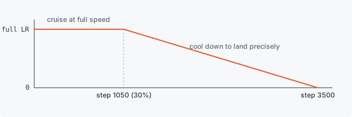
# learning rate schedule: stable then decay
def set_hparams(step, cooldown_frac=0.7):
    progress = step / train_steps
    assert 0 <= progress < 1
    if progress < 1 - cooldown_frac:
        eta = 1.0
    else:
        eta = (1 - progress) / cooldown_frac
    for opt in optimizers:
        for group in opt.param_groups:
            group["lr"] = group["initial_lr"] * eta

Full strength for the first 30% of training, followed by a linear ramp down to zero. Big steps help early while the model is far from good and moving in almost any direction is an improvement. Near the end, we shrink them so the model settles into a minimum instead of bouncing around it.

Part 6: The training loop

########################################
#        Training and Validation       #
########################################

for p in model.parameters():
    dist.broadcast(p.detach(), 0)
# start the clock
training_time = 0
dist.barrier()
t0 = time.perf_counter()

Final setup. The parameters were randomly initialized independently on each rank, so rank 0 broadcasts its values to everyone, guaranteeing all copies start identical.

Then, we start the stopwatch and go into the main loop.

for step in range(train_steps + 1):

    # --------------- VALIDATION SECTION -----------------
    if step == train_steps or step % 125 == 0:
        # stop the clock
        dist.barrier()
        training_time += time.perf_counter() - t0
        model.eval()
        val_loss = 0
        with torch.no_grad():
            assert len(val_inputs) % mbs == 0
            for i in range(len(val_inputs) // mbs):
                val_loss += model(val_inputs[i*mbs:(i+1)*mbs], val_targets[i*mbs:(i+1)*mbs])
        dist.all_reduce(val_loss, op=dist.ReduceOp.SUM)
        val_loss /= val_tokens
        print0(f"step:{step}/{train_steps} val_loss:{val_loss:.5f} train_time:{training_time:.3f}s"
               + f" step_avg:{1000*training_time/max(step, 1):.2f}ms", console=True)
        model.train()
        # start the clock again
        dist.barrier()
        t0 = time.perf_counter()

    if step == train_steps:
        break

The loop runs 3,501 times: 3,500 training steps, with a measurement pass every 125 steps and one final measurement at the very end (that last iteration measures and immediately breaks; no 3,501st training step happens).

The validation section computes the validation loss on the text we held out earlier. Notes:

• The stopwatch stops before validating and restarts after (with barriers so all ranks pause together). Only training time counts.
• model.eval() and the torch.no_grad() block switch off training bookkeeping (no gradient recording needed) while measuring; model.train() switches it back.
• Each rank measures its own slice of the 10.5 million validation tokens in chunks of 64 sequences; all_reduce sums the per-rank totals (all_reduce: every GPU contributes a value, every GPU receives the combined result), and dividing by the token count turns the summed cross-entropy into the reported per-token average.

    # --------------- TRAINING SECTION -----------------
    inputs, targets = next(train_loader)
    # accumulate across microbatches in case we are running with fewer than 8 gpus
    assert len(inputs) % mbs == 0
    for i in range(len(inputs) // mbs):
        model(inputs[i*mbs:(i+1)*mbs], targets[i*mbs:(i+1)*mbs]).backward()
    for name, p in model.named_parameters():
        assert p.grad is not None, name
        dist.all_reduce(p.grad, op=dist.ReduceOp.SUM)
    # set optimization hyperparameters and take a step
    set_hparams(step)
    for opt in optimizers:
        opt.step()
    model.zero_grad(set_to_none=True)
    approx_training_time = training_time + (time.perf_counter() - t0)
    print0(f"step:{step+1}/{train_steps} train_time:{approx_training_time:.3f}s"
           + f" step_avg:{1000*approx_training_time/(step + 1):.2f}ms", console=True, log=False)

The training section:

• Fetch the next batch of tokens. Each rank gets a slice.
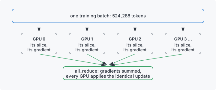
• The microbatch loop: each rank processes its sequences in chunks of mbs = 64, which is sized to fit in memory in an H100 GPU (80 GB). On 8 GPUs, each rank has exactly one chunk; on 1 GPU, it has eight. The .backward() call after each chunk makes gradients add up in the .grad fields.
• Once each GPU has a gradient from its own slice of the batch, dist.all_reduce(p.grad) adds those partial gradients together and gives the total back to every GPU. Each GPU ends up with the gradient for the full batch.
• Next, we update the scheduled learning rate and let both optimizers (AdamW and Muon) take their step.
• Then, model.zero_grad(set_to_none=True) clears the gradients for the next step (backward always adds, so they must be reset). set_to_none=True drops each .grad tensor to None rather than writing zeros, which saves some time.
• The last print is a progress heartbeat to console only.

dist.destroy_process_group()

The end. We've seen all 355 lines.

Takeaways

How does this script go from Karpathy's 19,560 learning steps to 3,500?⁴

It only took 355 lines of code on top of PyTorch, without any additional frameworks. And, most of the script is textbook. So, the speedup comes from:

1. An accumulation of small, empirically validated choices: QK norm, zero-init projections, soft-capped logits, squared ReLU, and tuned constants.
2. One genuinely new idea, the Muon optimizer (invented by Keller Jordan, the speedrun organizer).

The current record stands at 2,690 steps.

To go deeper into the tricks behind the fastest scripts, Damek Davis wrote a walkthrough of a recent wall-clock record: part I and part II; Tyler Romero maintains a living worklog explaining each record's technique. For the fundamentals in video form, watch Karpathy reproduce GPT-2 from an empty file, which started the whole thing.

Appendix: run it yourself on rented hardware

Here are the steps to run this script yourself and reproduce the 3.28-at-3,500-steps result.

1. Rent a machine. You want an 8× NVIDIA H100 instance (the speedrun's reference hardware; official records are timed on Prime Intellect instances, but Lambda and other clouds work equally well for unofficial runs). This costs roughly $20 per hour. Budget about an hour total including setup; the run itself is around 10 minutes. Pick an image with PyTorch 2.5 or later and CUDA preinstalled.

2. Get the data. The tokenized FineWeb shards are published alongside the speedrun repository, which includes a download script. The baseline consumes 1.835 billion tokens (3,500 steps × 524,288), which is 19 shards of 100 million tokens, plus the validation shard the script downloads automatically:

git clone https://github.com/KellerJordan/modded-nanogpt.git
cd modded-nanogpt
pip install -r requirements.txt
python data/cached_fineweb10B.py 19

The download is about 4 GB and typically takes a few minutes.

3. Get the script. Save train_gpt_simple.py into the repository root, next to the data folder.

4. Run it.

torchrun --standalone --nproc_per_node=8 train_gpt_simple.py

torchrun is the launcher discussed in Part 4: it starts 8 copies of the script and sets the environment variables through which they find their GPU and each other.

5. What you should see. A couple of minutes of compilation silence, then a validation line every 125 steps:

step:0/3500 val_loss:10.82584 train_time:0.000s step_avg:0.05ms
step:125/3500 val_loss:4.64566 train_time:20.580s step_avg:164.64ms
step:250/3500 val_loss:4.10409 train_time:38.846s step_avg:155.38ms
...
step:3500/3500 val_loss:3.27851 train_time:509.113s step_avg:145.46ms

The first line, before any training, sits near 10.8, which is exactly the loss of assigning equal probability to all 50,257 tokens (the natural logarithm of 50,257 is 10.82). The final validation loss should land just below 3.28.

Individual runs vary by random seed, so serious speedrun claims are checked across multiple runs.

Want to leave a comment? You can post under the linkedin post or the X post.

Footnotes

1. Karpathy's original script needed about 10B tokens to hit the same bar. ↩

2. Speedrun culture: even file reading is written so as to waste nothing. ↩

3. Some models reuse the embedding table for the output projection; this one keeps the two separate, which costs parameters but trains better here. ↩

4. The results from the wall-clock speedrun are more dramatic, going from 45 minutes to under 90 seconds. ↩