Training an AlphaZero-Style AI for a New Board Game
Here is part 2: Deep Dive: Inference Pipeline for Self-Play.
I created wallgame.io, an online board game. Since it's a two-player game, I wanted a human-level AI so anyone could play at any time.
I built a traditional, Minimax-based engine, while my friend Thorben built an AlphaZero-style AI: a neural network trained through self-play, guided by Monte Carlo Tree Search, running on a consumer GPU.
The AlphaZero engine turned out to be much stronger. Based on the experiment, I'd recommend anyone wanting to add a strong engine to their own game to follow the AlphaZero route.
This post describes the design and can serve as a reference. We cover the architecture, implementation, training, and server integration.
Links
- The game and the AlphaZero-based AI are live at wallgame.io. If you manage to beat the Hard Bot, let me know!
- Thorben's original engine: Deep-Wallwars. Credits to him for re-implementing the AlphaZero paper from scratch!
- The game has a monorepo with:
- Server
- Frontend
- Bot client
- Updated version of Thorben's engine
- A dummy engine for testing
- The game has a dev blog, nilmamano.com/blog/category/wallgame including this post.
- The minimax-based C++ engine can be played against in the old site: wallwars.net.
- References: the AlphaZero paper by Silver et al. (2017) and the ResNet paper by He et al. (2015).
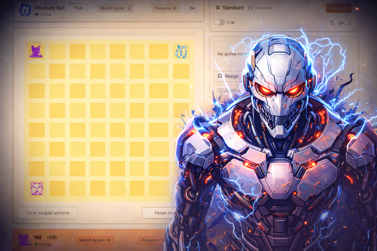
The Wall Game
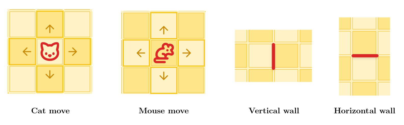
The Wall Game is a turn-based game played on a rectangular grid. Each player controls a cat and a mouse, which start at the corners, and the goal is to catch the opponent's mouse before they catch yours.
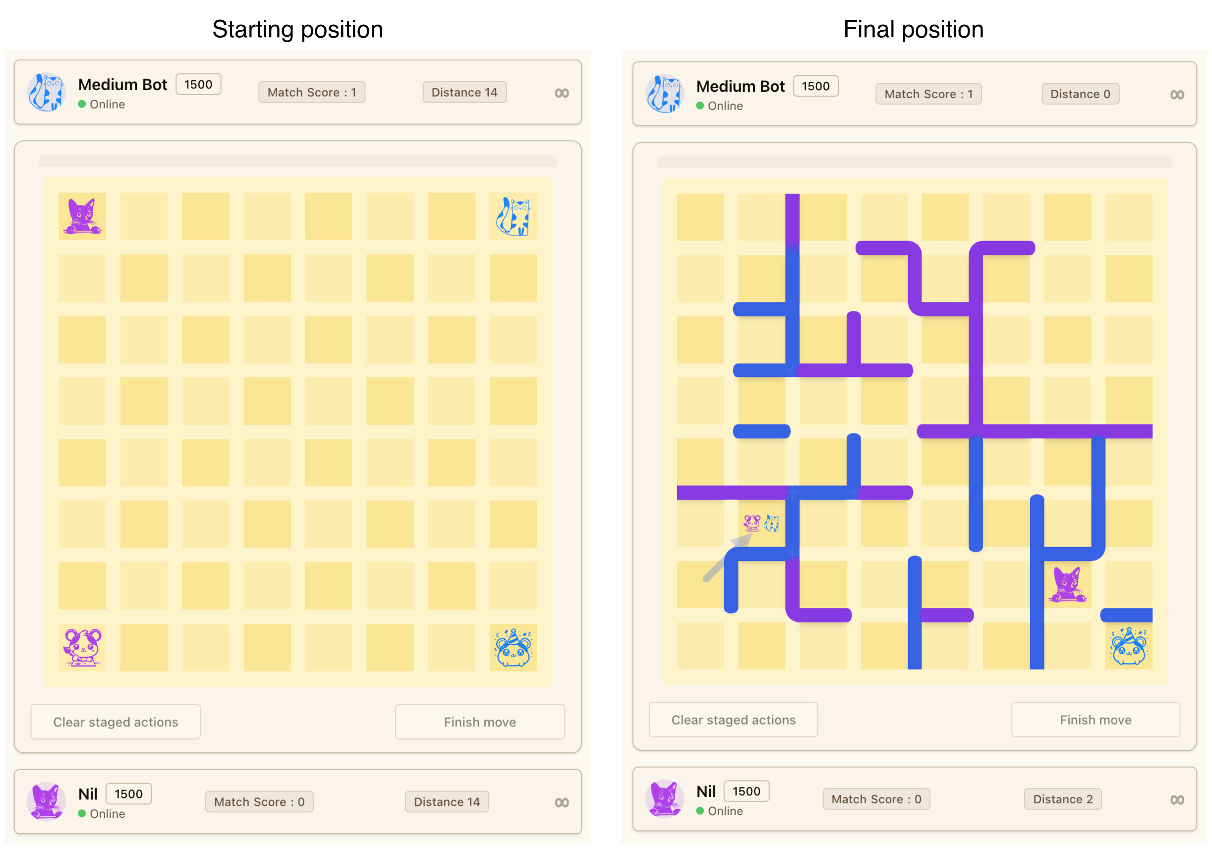
On each turn, you take 2 actions. Each action can be moving your cat, moving your mouse, or placing a wall. Cats and mice move to adjacent cells, but walls can be placed between any two cells on the board. The only restriction is that you cannot completely block the opponent's cat from reaching your mouse. The full rules are at wallgame.io/learn.
Watch this replay of a full game to get a feel for the tactics that emerge. You can see more games in action in the landing page's game showcase (wallgame.io).
Why it is Hard for AI
Like chess and Go, decisions have long-term consequences. A wall placed on move 5 might not matter until move 25, when it blocks a critical escape route. This makes it difficult to write a good handcrafted evaluation function - the kind of approach that powered chess engines for decades.
For the Minimax engine, I implemented all the classic techniques: alpha-beta pruning, transposition tables, and even some clever graph theory algorithms for efficient move generation, but it doesn't scale.
What crushed it is the branching factor. On an RxC board, there are about 2*R*C possible walls. With two actions per turn, the number of possible moves is roughly the square of that.
In contrast, the AlphaZero-based engine is superhuman on 8x8 boards, handling raw branching factors of approximately (2*8*8 + 8)^2 = 18496. I'm now training models for boards up to 10x12. Chess has average branching factor ~40.
This is exactly the kind of problem where Monte Carlo Tree Search (MCTS) with a learned evaluation function through self-play shines.
The AlphaZero Recipe
In 2017, DeepMind's AlphaZero showed a different path. Instead of hand-engineering the evaluation function, AlphaZero trains a neural network to learn it from scratch. The network starts knowing nothing about the game except the rules and improves by playing against itself thousands of times.
It's this flexibility that makes the recipe plug-and-play for new games.
The system has three components that work together in a loop:
Monte Carlo Tree Search (MCTS)
MCTS is the search algorithm. Given a board position, it repeatedly explores possible future moves, building a search tree of board positions. At each node, it must decide which move to explore next - this is where the neural network comes in. MCTS uses the network's predictions to focus on the most promising moves rather than searching blindly. After exploring enough positions, it picks the move with the most supporting evidence.
MCTS faces a classic exploration-exploitation tradeoff: among the possible moves, how much time should it spend exploring each? Should it focus on the best moves found so far (exploitation), or try alternatives that seem unpromising but could turn out to be good (exploration)?
AlphaZero follows an elegant solution known as Upper Confidence Bound (UCB). To use UCB, for each option, you need two things: the expected payoff and the expected variance (in MCTS, we estimate those based on visit counts and average evaluation). The option with the highest payoff maximizes exploitation; the one with the most variance maximizes exploration.
To balance the two, pick the option maximizing expected payoff + one standard deviation. This way, as MCTS explores a move further and its variance goes down, less explored moves become more attractive.
The basic MCTS loop starts with an empty tree where the root represents the current position. We then collect a given number of "samples" (usually 1k+).
Each sample walks down the tree, using UCB to choose moves, until it reaches a position that has not been evaluated yet. The neural network evaluates it and the result is backpropagated: for each ancestor position, we update the visit count and the average evaluation. This information refines the UCB of all ancestors.
The Neural Network
The neural network takes a board position as input and produces two outputs:
- A policy: a probability distribution over all legal moves, representing how promising each one looks.
- An evaluation: a single number between -1 and +1, estimating who's winning.
The policy guides MCTS toward promising moves. The evaluation replaces the classic handcrafted evaluation function. Together, they keep the search time from blowing up with the branching factor.
The Self-Play Training Loop
We start with a random neural network (more on architecture later) and train it in generations. Here are some numbers from one of our training runs.
- Each generation is 4,000 self-play games.
- Each game lasts around 40 turns (80 moves or 'plies').
- Each player must take 2 actions per ply.
- For each action, we collect 1200 MCTS samples.
- Each sample plays the game forward until it reaches a new position, which is evaluated with a model inference.
That comes out to about 80 * 2 * 1200 = 192k inferences per game, for a total of 4000 * 192k = 768M inferences per generation.
We'll later touch on the optimizations that make this doable: coroutines, batching, and caching.
After each self-play game, the moves chosen by MCTS (each based on 1200 samples) and the game outcome become training data. The network learns to predict which moves MCTS would choose (policy) and who won (value).
After each generation, we train the network on the accumulated data from the few latest generations. The updated network is used for the next generation of self-play, producing better data, which produces a better network, and so on.
For the first generation, we used a simple bootstrap policy: cats walked toward the opponent's mouse while placing a few random walls so the model learns that it's an option.

Neural Network Architecture
Our network follows the AlphaZero architecture: a ResNet core with 20 residual blocks and 128 hidden channels, totaling about 2.3 million parameters. Small by modern deep learning standards, but large enough to capture the strategic complexity of an 8x8 board game.
ResNet was designed for image classification, using convolutions to extract local features. This works well for board games like chess or the Wall Game because (1) the board is a grid, like an image, and (2) local features matter - like clusters of adjacent walls blocking a path.
Input Encoding
The network sees the board as 8 "planes" (like color channels in an image), each the size of the board:
| Plane | What it Represents | Values |
|---|---|---|
| 0 | Distance from your cat to every cell | 0 at cat's position; less than 1 for reachable cells, increasing with distance; 1 for unreachable cells |
| 1 | Distance from your mouse to every cell | Same as above, from mouse's position |
| 2 | Distance from opponent's cat to every cell | Same as above, from opponent's cat |
| 3 | Distance from opponent's mouse to every cell | Same as above, from opponent's mouse |
| 4 | Vertical walls | 1 if the right edge of this cell is blocked, 0 otherwise |
| 5 | Horizontal walls | 1 if the bottom edge of this cell is blocked, 0 otherwise |
| 6 | Second action indicator | All 0s during first action, all 1s during second action |
| 7 | Current player indicator | All 1s if current player is P1, all 0s if P2 |
A key design choice is using relative distances rather than raw positions for the first four planes. Instead of a single "1" at the pawn's location, every cell gets a value representing its distance from the pawn (computed via BFS through the current wall layout). This encoding is more informative - the network immediately "sees" how walls affect reachability - and generalizes better across positions.
Before the residual blocks, an initial convolution lifts from the 8 input planes to 128 hidden channels. Then, each of the 20 residual blocks applies:
- A
3x3convolution (128 -> 128 channels), followed by batch normalization and ReLU activation. - Another
3x3convolution (128 -> 128 channels), followed by batch normalization. - Add the original input of the block back in (the residual connection), then apply ReLU.
All convolutions preserve the spatial dimensions - the board stays rows x cols through the network. They also omit the bias term, since batch normalization already includes a learnable shift that serves the same purpose.
The residual/skip connection in step 3 is what makes it possible to train 20+ layers deep. As explained in the classic ResNet paper, by adding the input back, gradients can flow directly through the skip connection during training, preventing the "vanishing gradient" problem.
Output Heads
The network has two output heads branching from the shared ResNet body:
Policy head: Outputs a probability for each legal action - one for each wall placement (2 x cols x rows, for vertical and horizontal walls) plus 4 cat move directions (up, down, left, right). A softmax ensures all probabilities sum to 1.
In the initial 8x8 model we trained, there are no outputs for mouse moves - it was trained for the Classic variant, where mice are fixed in the corners. This will be relevant later when we discuss adapting the model for other variants.
Value head: A single number passed through tanh, giving a value in [-1, +1]. Positive means the current player is winning; negative means losing.
Training Loss
The loss function has two parts:
- KL divergence between the network's policy output and MCTS's move probabilities (derived from visit counts in the search tree). This teaches the network to predict which moves MCTS would choose.
- Mean squared error between the network's value output and the actual game outcome. This teaches the network to predict who wins.
The idea is that the model slowly converges to match the policy and evaluation computed by MCTS, so a single model evaluation approximates an MCTS search with 1000+ samples.
Pseudocode
Here's a simplified view of the architecture:
ResNet(input: 8 x rows x cols):
    x = Conv2d(8 -> 128, 3x3) -> BatchNorm -> ReLU

    for each of 20 residual blocks:
        residual = x
        x = Conv2d(128 -> 128, 3x3) -> BatchNorm -> ReLU
        x = Conv2d(128 -> 128, 3x3) -> BatchNorm
        x = ReLU(x + residual)      ← skip connection

    policy = Conv2d(128 -> 32, 3x3) -> BatchNorm -> ReLU -> Flatten
           -> Linear(32·rows·cols -> 2·rows·cols + 4) -> Softmax

    value = Conv2d(128 -> 32, 3x3) -> BatchNorm -> ReLU -> Flatten
          -> Linear(32·rows·cols -> 1) -> Tanh

    return policy, value
Making MCTS Fast: Coroutines, Batching, Caching
The self-play phase is the performance bottleneck. Training the network between generations is relatively fast.
Our superhuman model was trained on 750k self-play games over many generations, taking about 100 hours on a single RTX 5080 - over 1 billion neural network evaluations per hour.
The GPU Utilization Bottleneck
Our goal during self-play is to maximize GPU utilization.
TensorRT (NVIDIA's optimized inference runtime) loads the model into GPU memory at initialization time, and then it sits waiting for positions to evaluate.
The GPU can evaluate many positions in parallel, so the key is sending multiple at a time. We found that batches of 256 are enough to reach ~100% GPU utilization. Without batching, GPU I/O becomes the bottleneck.
Parallel samples
The standard MCTS loop is inherently sequential: traverse the tree, reach a leaf, evaluate it, backpropagate, repeat. Each iteration depends on (or at least benefits from) the previous ones, because the tree becomes more refined after each sample. Naively, we'd evaluate one position at a time - no batching.
During self-play, we can play 256+ games in parallel (using a CPU thread pool - more on that later), which fills the batches without needing parallel samples for the same game.
However, parallel samples for a single game can be valuable:
- When playing against the model, for maximum strength, we'd want good GPU utilization even for a single game.
- During self-play, having fewer games is better for caching (the cache is shared across games) and for memory utilization (so we don't need to store 256+ MCTS trees).
Therefore, it's worth supporting parallel samples. In the ideal case, parallel samples go down different paths, updating different parts of the search tree. However, parallel samples may reach the same leaf node, duplicating work. To avoid this, when a sample goes down a branch, it temporarily and artificially lowers the UCB of nodes along the path, so other samples avoid that branch (this is called "virtual loss").
Since multiple samples update the tree concurrently, node statistics use atomic updates to stay consistent.
Coroutine-Based Parallelism
Our approach uses C++ coroutines (via Facebook's Folly library) to decouple MCTS traversal from neural network evaluation.
Each sample - whether a parallel sample within one game or across multiple self-play games - is a coroutine: a lightweight function that can suspend and resume. When a coroutine reaches a leaf node and needs a neural network evaluation, it doesn't block. Instead, it submits its request to a shared queue and suspends, freeing the thread for other coroutines.
A dedicated batch worker thread monitors the queue. When enough requests accumulate (or a short timeout expires), it collects them into a batch - typically 256 positions - and sends the batch to the GPU in a single TensorRT call. When the GPU returns results, each waiting coroutine resumes with its result.
A relatively small thread pool is enough to keep the GPU at 100% utilization, since the MCTS traversal is computationally lightweight.
Main
    │
    v
Thread pool (Folly's CPUThreadPoolExecutor)
    │
    ├── MCTS Coroutine 1: traverse tree -> reach leaf -> [suspend, enqueue request]
    ├── MCTS Coroutine 2: traverse tree -> reach leaf -> [suspend, enqueue request]
    ├── MCTS Coroutine 3: backpropagating result (resumed)
    ├── ...
    │
    v
Inference request queue (Folly's lock-free MPMC)
    │
    v
Batch worker thread
    │ collects 256 requests
    v
GPU (TensorRT)
    │ returns 256 results
    v
Resume suspended coroutines with results
This keeps both CPU and GPU busy simultaneously. 20+ CPU threads constantly traverse trees and backpropagate results, while the GPU processes large batches of evaluations. The lock-free MPMC (Multi-Producer Multi-Consumer) queue from Folly handles the handoff without expensive synchronization.
Caching
All model evaluations go in an LRU cache (folly::EvictingCacheMap). Since multiple threads read and write concurrently, the cache is sharded by position hash, with each shard having its own lock. This reduces contention. We keep the number of shards roughly equal to the thread pool size.
Tree reuse
After each move, we don't discard the MCTS tree. The chosen move has likely been explored to some depth, so we reuse it.
We shift the root down to the chosen move's subtree, and then free memory for all parts of the tree unreachable from the new root.
Key MCTS Parameters
A few parameters govern how MCTS explores the game tree:
- PUCT constant (2.0): Controls the exploration-exploitation tradeoff. Higher values explore more broadly; lower values focus on the most promising moves.
- Dirichlet noise (α=0.3, factor=0.25): Random noise added to the root node's prior probabilities. This ensures self-play games explore diverse strategies rather than always playing the same opening.
- Max parallelism (more = stronger play / faster MCTS exploration): How many MCTS samples can run concurrently for a single game session. Too many and they interfere with each other (exploring redundant branches); too few and the GPU may go hungry (if there aren't enough parallel games).
Self-play parameters
During self-play, we have to decide how many parallel games to run and how many parallel samples per game. There is a tradeoff:
- Parallel games are bad for caching and memory usage (storing the MCTS for each game, though MCTS trees are relatively small)
- Parallel samples are bad for MCTS performance, because each sample benefits from previous ones.
We tweak these parameters to find a good balance that keeps the GPU fully utilized.
Training
Thorben started small with a 5x5 board to validate the pipeline end-to-end before investing compute.
With the pipeline validated, he scaled to the 8x8 board.
Training setup:
- Games per generation: 5,000
- MCTS samples per action: 1,200
- Training window: last 20 generations (~100k most recent games)
- Total training time: ~100 hours
The first generation used a simple heuristic policy (walk toward goal, place walls randomly) instead of the neural network to bootstrap initial training data. Random self-play would produce games that meander aimlessly - it's hard for a cat to randomly walk into a mouse, so games would drag on and the signal-to-noise ratio would be too low for the network to learn anything useful. The heuristic bootstrap gives it a foundation: "moving toward the opponent's mouse is good."
Evaluating model strength
How do we know when to stop training?
Decreasing validation loss doesn't necessarily mean the model is getting stronger. It could mean that both the tree search and neural network converged on a suboptimal strategy.
A good ad-hoc way to test model strength is to play against it.
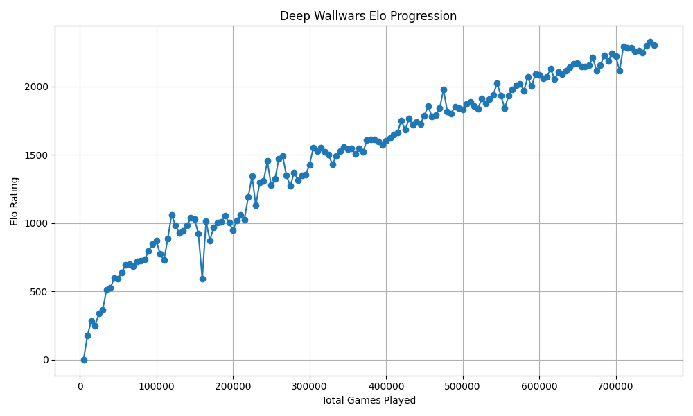
A more rigorous way is to make all generations play against each other and use Elo to rank them.
After 750,000 self-play games, the result is a superhuman player that moves almost instantly, even though the Elo didn't stagnate yet. Its style is recognizably strategic but unpredictable to me and other "strong" human players.
New Variant: 8x8 Standard
As mentioned earlier, this first model was trained for the "Classic" variant, where mice are fixed in the corners.
With a strong Classic model in hand, I turned to Standard - the variant where each player also controls the mouse and can try to run away from the opponent's cat.
Standard needs 8 pawn-move channels (4 for the cat, 4 for the mouse) instead of Classic's 4, so we had to train a new model with a wider policy head.
Rather than training from scratch, I warm-started it with the Classic model's weights. Wall placement patterns, spatial reasoning, and basic strategy transfer between variants - only mouse-handling needs to be learned from scratch.
This mostly worked, but at first the model showed a funny holdover from Classic training: the cat would move to the corner where the mouse spawns instead of the mouse itself. Even if the mouse was right next to it, it'd ignore it and head for the corner.
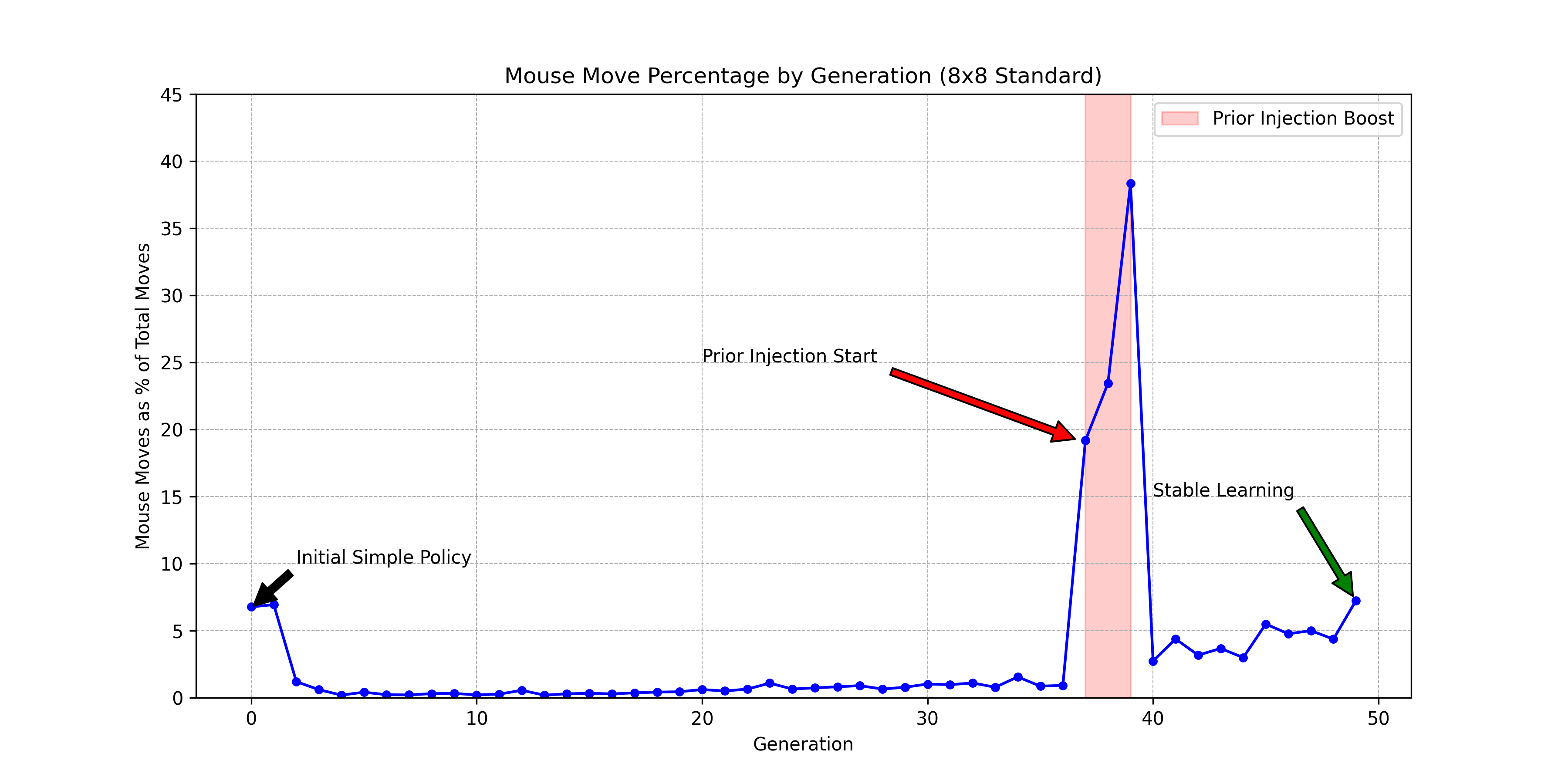
A bigger issue was a cold-start problem: the model never moved its mouse. Mouse move priors started with random values but got stuck so low that MCTS never explored them. Since MCTS never explored mouse moves, the training data never contained them, so the network never learned their value.
Our fix was pragmatic: for a few generations, we boosted mouse-move probabilities in the MCTS policy, forcing the search to explore them even though the network rated them unlikely. Once the training data contained enough mouse-move examples, the network started learning their value on its own, and we removed the boost.
The warm-start paid off: the model became strong in far fewer generations.
The Universal Model
Next, I wanted models that could play the standard and classic variants for larger boards (up to 12x10).
Warm-starting across board sizes is possible - the core ResNet convolutions are input-size independent and can still detect wall patterns regardless of board size. The Linear layers in the output heads need remapping, but that's a small fraction of the network.
The question is: which models should we warm-start from?
We could do 8x8 Standard -> 12x10 Standard and 8x8 Classic -> 12x10 Classic, or perhaps 8x8 Classic -> 12x10 Classic -> 12x10 Standard.
But training multiple models feels wasteful - everything is done twice, once per variant.
My most ambitious training experiment is the universal model: a single network that plays both Classic and Standard on larger boards (12x10), so all compute goes toward improving one model.
This required several changes:
- New variant plane: A new input plane (plane 8) indicates the variant (
0everywhere for Classic,1everywhere for Standard). - Spatial remapping for warm-start: The 12x10 board is larger than the 8x8 model we're warm-starting from. Convolutional layers transfer directly (input-size independent), but the Linear layers in the output heads are tied to specific board positions. We spatially embedded the 8x8 weights within the 12x10 grid, centering them with an offset of (col=2, row=1), and randomly initialized weights for the new boundary positions.
12 columns x 10 rows:

    col: 0  1  2  3  4  5  6  7  8  9  10 11
row 0:  .  .  .  .  .  .  .  .  .  .  .  .   <-- new
row 1:  .  . [X][X][X][X][X][X][X][X] .  .    \
row 2:  .  . [X][X][X][X][X][X][X][X] .  .     |
row 3:  .  . [X][X][X][X][X][X][X][X] .  .     |
row 4:  .  . [X][X][X][X][X][X][X][X] .  .     | 8x8 embedded
row 5:  .  . [X][X][X][X][X][X][X][X] .  .     |
row 6:  .  . [X][X][X][X][X][X][X][X] .  .     |
row 7:  .  . [X][X][X][X][X][X][X][X] .  .     |
row 8:  .  . [X][X][X][X][X][X][X][X] .  .    /
row 9:  .  .  .  .  .  .  .  .  .  .  .  .   <-- new
- Progressive unfreezing: After warm-starting, we froze the convolutional body for the first few generations, training only the linear head layers. This prevents catastrophic forgetting - without freezing, the high loss from randomly-initialized boundary weights would generate large gradients that destroy the features learned on 8x8.
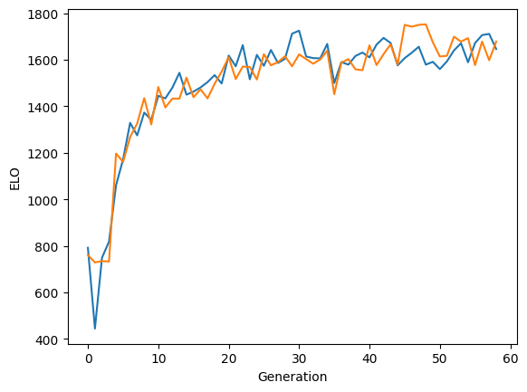
- Half-and-half self-play: Each generation plays half its games as Classic and half as Standard. The variant indicator (plane 8) tells the network which variant it's playing, ensuring the model learns to use that signal from the start. The strength for the two variants evolved at a similar pace:
As of Feb 2026, the universal model makes good moves early, but sometimes plays nonsensically later in the game. It's already live on the site, but I'm still training it further.
Board Padding: One Model, Many Board Sizes
Models are trained for a specific board size (e.g., 8x8), but the same model can be used for smaller boards too.
Rather than training separate models for each board size, we embed smaller boards inside the model's fixed grid using padding walls.
For example, to play on a 6x6 board with an 8x8 model, we place the 6x6 game area inside the 8x8 grid and surround the unused border cells with walls. The engine sees an 8x8 board where some areas are walled off - from its perspective, the padding walls are just more walls.
The question was whether this works without explicit training on padded boards - walls forming a complete border around a smaller subgrid don't come up in natural gameplay.
Thankfully, the model's pattern recognition is general enough, so this worked out of the box (pun intended).
Serving Moves in a Live Web Game
After training a strong model, the next challenge is serving it to players.
Deployment strategies
For the Minimax-based engine, which can be played against on the old site, I compiled the C++ engine to WebAssembly and shipped the wasm with the frontend, so it runs on your browser. This has some downsides:
- Not all browsers support wasm (especially on phones)
- Transposition tables require quite a bit of memory.
- Engines that require a GPU - like AlphaZero - aren't an option for the browser.
Another option is to host the server on a machine with a GPU. The downside is that providers offering GPU compute are significantly more expensive than regular servers.
I chose a third option: run the engine on my home machine (RTX 4090) and keep a long-lived WebSocket connection to the server.
The inference batching architecture we described in the self-play section can also be used to batch inference requests for multiple live games vs human players. Thanks to this setup, the server should be able to handle 100 concurrent players easily.
The Integration Challenge
The server and the engine talk through a custom protocol. The architecture has three systems that need to communicate:
- The server: a Hono/Bun application running on Fly.io, handling game logic, matchmaking, and WebSocket connections to browser clients. No GPU.
- The bot client: a TypeScript process running on a Linux machine with a GPU. Manages the connection between the server and the engine.
- The engine: the C++ binary. Loads models into GPU memory, maintains MCTS trees, and evaluates positions.
For now, the server runs on a single machine. This matters because the bot connects to one machine - if players hit a different one, they couldn't reach the bot. (I wrote a post about how Lichess handles multi-server scaling.)
The bot client automatically reconnects, so the official bots stay available even across server deploys.
The bot client is engine-agnostic - it's configured with a CLI command to start the engine, and then communicates via stdin/stdout with JSON objects.
Anyone can reuse the bot client and plug in their own engine.

The system also powers an evaluation bar - a live position evaluation display (like those on chess streaming sites) that players and spectators can toggle during a game.
The Protocol
Stateless vs long-lived engines
The first bot protocol was simple: for each move request, spawn a fresh engine process, pipe in a JSON request via stdin, read the response from stdout, kill the process.
This works, but doesn't leverage the strengths of MCTS:
- Loading a TensorRT model into GPU memory takes longer than the computation itself.
- The MCTS tree and the evaluation cache are not reused between turns.
I moved to a long-lived process: the engine starts once, loads the models into GPU memory once, and handles requests over a JSON-lines protocol (one JSON object per line on stdin/stdout).
The main concept in the protocol is the Bot Game Session (BGS): a stateful context for one game, with its own MCTS tree living in memory.
Multiple BGSs can run concurrently, sharing the GPU through the same batched inference pipeline used during training.
The BGS protocol consists of only 4 messages:
- When a game starts, the server sends
start_game_session. The engine creates a new MCTS tree. - When the server needs a move, it sends
evaluate_position. The engine runs MCTS against its existing tree and returns a move and evaluation (the search goes two levels deep, since one move consists of two actions). - When the server (the authoritative source for game state) determines that a move was made, it sends
apply_move. The engine updates the MCTS tree - pruning it as during self-play: the subtree rooted at the played move becomes the new root, preserving relevant search work. - When the game ends,
end_game_sessioncleans up.
The protocol could be extended to support features like draws, but for simplicity we don't yet. The server auto-rejects draw offers on behalf of bots.
Takebacks are also handled by the server. It ends the current BGS, starts a fresh one, and replays the moves up to the new position. This complexity is hidden from the bot client - it sees the same four message types.
An expectedPly field in each request prevents race conditions - if a stale evaluation request arrives after a move has been applied, the ply mismatch catches it.
Bots as first-class citizens
Originally, starting a game against the AI gave you a token that you'd pass to the bot client to connect it to that specific game. This meant copy-pasting a token and re-running the bot client for every match.
Now, bots connect proactively to the server, and any connected bots appear in a bot table visible to all browser clients. Anyone can play against connected bots (they can also be made private for testing).
I use a special secret token to mark my own bot (running on my machine) as "official", which gets special labeling in the UI and tells the server to use it for the evaluation bar.
The Bot Client
The bot client is a TS process running on the GPU machine. It handles:
- WebSocket management: Maintains a persistent connection to the game server with automatic reconnection (exponential backoff with jitter). On startup, it registers which bots are available, what variants they support, and what board sizes they can play.
- Engine lifecycle: Spawns the engines on startup and keeps them running. If the WebSocket disconnects and reconnects, the engines stay alive - active game sessions continue seamlessly.
- Session multiplexing: Routes BGS messages between server and engines, multiplexing concurrent game sessions over each engine process.
The bot client is configured via a JSON file that specifies the bot's name, appearance (avatar, colors), engine parameters, and a command to launch the binary for each engine. This is what makes it engine-agnostic. Here is the official bot's config.
The Eval Bar
The eval bar is a live display showing the engine's position evaluation for every move. It works for bot games, human-vs-human games (unrated), live spectators, and past game replays.
For live games, the server maintains a BGS history: an evaluation for every position from game start. When a player or spectator toggles the eval bar, the server sends the full history to the frontend, providing instant evaluations for all past moves.
If a user fetches a past-game replay, or the eval bar is toggled mid-game for a non-bot game, the server replays all moves through the engine - sending evaluate_position and apply_move for each - to build the complete history before streaming it. This is invisible to the user; evaluations simply appear after a bit of delay.
What's Next
I'm working on a background process that analyzes past games played on the site and identifies positions that make for interesting puzzles. Instinctively, a puzzle-like position is one where there is a short tactical sequence that yields a decisive advantage. A good heuristic for whether a move is non-obvious is that the human player in the actual game didn't find it. To operationalize this, we can lean on the superhuman engine.
Imagine that you feed a position to the engine. At first, the evaluation is erratic, which is common, but then it settles around +0 (neutral position). After 10 seconds, however, the evaluation jumps to 80% winning for the player to move. That's an indication that the engine found a non-obvious good move.
Want to leave a comment? You can post under the linkedin post or the X post.